Trace Forward

Perform forward tracing of magnetic field lines.

This example demonstrates how to use the run_forward_tracing() function to trace magnetic field lines forward from a set of default starting points. It also shows how to load magnetic field data files and visualize the traced field lines in 3D.

import matplotlib.pyplot as plt

from mapflpy.scripts import run_forward_tracing
from mapflpy.utils import plot_traces
from mapflpy.data import fetch_cor_magfiles

Load in the magnetic field files

The fetch_cor_magfiles() function returns a tuple of file paths corresponding to the radial, theta, and phi components of the magnetic field data.

magnetic_field_files = fetch_cor_magfiles()

Run forward tracing using the default launch points

Note

By default, if no launch points are provided, the function will use a set of 128 predefined launch points distributed in a Fibonacci lattice at a radius of 1.01 Rsun.

traces = run_forward_tracing(*magnetic_field_files, context=CONTEXT)
print("Geometry shape:", traces.geometry.shape)

Geometry shape: (2000, 3, 128)

The shape of the resulting traces geometry is an M x 3 x N array, where M is the field line length (i.e. the buffer_size), N is the number of launch points (here 128), and the second dimension corresponds to the radial-theta-phi coordinates.

The utility functions provided in utils are designed to work with this contiguous memory layout for efficient processing and visualization.

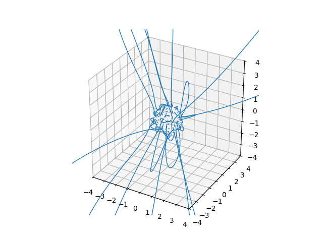
Plot traces using the plot_traces() utility function and adjust the field of view to be 4 Solar Radii in each direction

ax = plt.figure().add_subplot(projection='3d')
plot_traces(traces, ax=ax)

FOV = 4.0  # Rsun
for dim in 'xyz':
    getattr(ax, f'set_{dim}lim3d')((-FOV, FOV))
ax.set_box_aspect([1, 1, 1])

plt.show()