Manipulating Field Data

Pass in and manipulate in-memory magnetic field data

Attention

The Tracer class enforces a singleton pattern to manage issues that arise from the underlying mapflpy_fortran object not being thread-safe. As a result, it is recommended to use the Tracer class in single-threaded contexts only viz. instantiating one instance of the class at a time.

import matplotlib.pyplot as plt
import numpy as np
from psi_io import read_hdf_by_index

from mapflpy.tracer import Tracer
from mapflpy.utils import plot_traces, fetch_default_launch_points
from mapflpy.data import fetch_cor_magfiles

Load in the magnetic field files

The fetch_cor_magfiles() function returns a tuple of file paths corresponding to the radial, theta, and phi components of the magnetic field data.

magnetic_field_files = fetch_cor_magfiles()

The Tracer class is, for demonstration purposes, instantiated without arguments to illustrate how to set the magnetic field files post-initialization.

tracer = Tracer()

Here we use psi-io to read in the magnetic field data into memory as NumPy arrays, and then assign them to the respective attributes of the Tracer instance.

Note

When no *args are passed to the read_hdf_by_index() function, it reads in the entire dataset. For typical MAS magnetic field files, this results in a tuple where:

• the first element is the 3D array of magnetic field values (Fortran ordered),

• the subsequent elements are the scale arrays (r, theta, phi).

br = read_hdf_by_index(ifile=magnetic_field_files.br)
bt = read_hdf_by_index(ifile=magnetic_field_files.bt)
bp = read_hdf_by_index(ifile=magnetic_field_files.bp)

tracer.br = br
tracer.bt = bt
tracer.bp = bp

Using default launch points, perform forward tracing of magnetic field lines.

launch_points = fetch_default_launch_points(n=256)
traces = tracer.trace_fwd(launch_points=launch_points)

Plot traces using the plot_traces() utility function and adjust the field of view to be 20 Solar Radii in each direction.

ax = plt.figure().add_subplot(projection='3d')
plot_traces(traces, ax=ax, color='c')

FOV = 20.0  # Rsun
for dim in 'xyz':
    getattr(ax, f'set_{dim}lim3d')((-FOV, FOV))
ax.set_box_aspect([1, 1, 1])

plt.show()

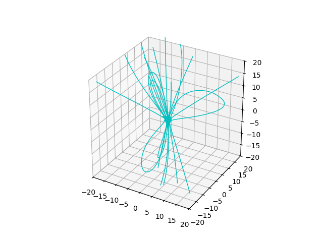
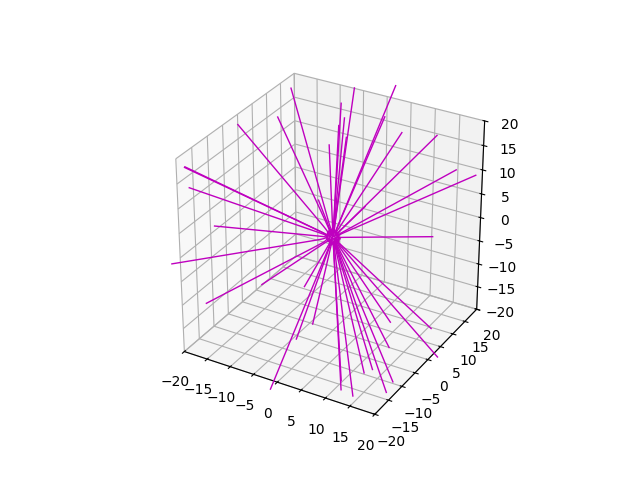
Now, we can manipulate e.g. the radial component of the magnetic field data – radially scaling the field by the square of the radius, and retracing from the same launch points.

new_br = br[0] * br[1] ** 2
tracer.br = new_br, *br[1:]
traces = tracer.trace_fwd(launch_points=launch_points)

ax = plt.figure().add_subplot(projection='3d')
plot_traces(traces, ax=ax, color='m')

FOV = 20.0  # Rsun
for dim in 'xyz':
    getattr(ax, f'set_{dim}lim3d')((-FOV, FOV))
ax.set_box_aspect([1, 1, 1])

plt.show()

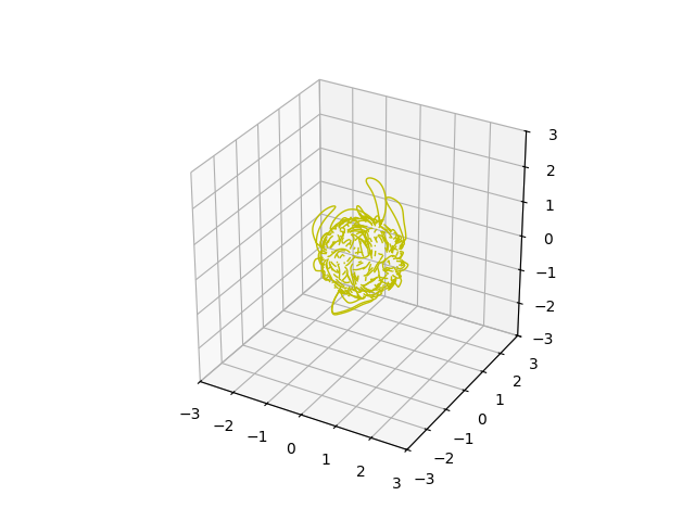
Next, we manipulate the radial component of the magnetic field data by diminishing weaker field regions by a factor of 4, and retracing from the same launch points.

new_br = np.where(abs(br[0]) < 1, br[0] * .25, br[0])
tracer.br = new_br, *br[1:]
traces = tracer.trace_fwd(launch_points=launch_points)

ax = plt.figure().add_subplot(projection='3d')
plot_traces(traces, ax=ax, color='y')

FOV = 3.0  # Rsun
for dim in 'xyz':
    getattr(ax, f'set_{dim}lim3d')((-FOV, FOV))
ax.set_box_aspect([1, 1, 1])

plt.show()