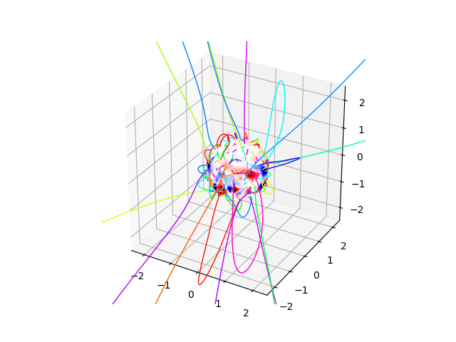
Adding a Magnetogram

Perform forward tracing of magnetic field lines and adding a magnetogram.

This example demonstrates how to use run_forward_tracing() and plot_traces() function to plot magnetic field lines, along with plot_sphere() to add a magnetogram at the solar surface.

from psi_io import np_interpolate_slice_from_hdf
import matplotlib.pyplot as plt
import matplotlib
import numpy as np

from mapflpy.scripts import run_forward_tracing
from mapflpy.utils import plot_traces, plot_sphere
from mapflpy.data import fetch_cor_magfiles

Load in the magnetic field files

The fetch_cor_magfiles() function returns a tuple of file paths corresponding to the radial, theta, and phi components of the magnetic field data.

magnetic_field_files = fetch_cor_magfiles()

Run forward tracing using the default launch points

Note

By default, if no launch points are provided, the function will use a set of 128 predefined launch points distributed in a Fibonacci lattice at a radius of 1.01 Rsun.

traces = run_forward_tracing(*magnetic_field_files, context='fork')
print("Geometry shape:", traces.geometry.shape)

Geometry shape: (2000, 3, 128)

The shape of the resulting traces geometry is an M x 3 x N array, where M is the field line length (i.e. the buffer_size), N is the number of launch points (here 128), and the second dimension corresponds to the radial-theta-phi coordinates.

The utility functions provided in utils are designed to work with this contiguous memory layout for efficient processing and visualization.

psi-io np_interpolate_slice_from_hdf() is used to linearly interpolate a 2D slice of data at the solar surface (r=1.0 Rs), using the radial component of the magnetic field.

Note

Currently there is no documentation website for the psi-io package, but the source code is available for further inspection at predsci/psi-io

values, theta_scale, phi_scale = np_interpolate_slice_from_hdf(1.0, None, None,
                                                               ifile=magnetic_field_files.br)

Plot traces using the plot_traces() utility function and adjust the field of view to be 2.5 Solar Radii in each direction

rsample = np.random.random_sample(size=traces.geometry.shape[-1])
colors = matplotlib.colormaps['hsv'](rsample)

ax = plt.figure().add_subplot(projection='3d')
plot_sphere(values, 1.0, theta_scale, phi_scale, clim=(-10, 10), ax=ax)
plot_traces(traces, ax=ax, colors=colors)
FOV = 2.5  # Rsun
for dim in 'xyz':
    getattr(ax, f'set_{dim}lim3d')((-FOV, FOV))
ax.set_box_aspect([1, 1, 1])

plt.show()