Adjusting mapfl Parameters

Adjust the default mapfl parameters

This example demonstrates how to use the Tracer class to perform fieldline tracing using non-default mapfl parameters. Furthermore, it explores the “Tracer as dictionary” design pattern to update mapfl parameters after instantiation.

Attention

The Tracer class enforces a singleton pattern to manage issues that arise from the underlying mapflpy_fortran object not being thread-safe. As a result, it is recommended to use the Tracer class in single-threaded contexts only viz. instantiating one instance of the class at a time.

import matplotlib.pyplot as plt
import numpy as np

from mapflpy.tracer import Tracer
from mapflpy.utils import plot_traces
from mapflpy.data import fetch_cor_magfiles

Load in the magnetic field files

The fetch_cor_magfiles() function returns a tuple of file paths corresponding to the radial, theta, and phi components of the magnetic field data.

magnetic_field_files = fetch_cor_magfiles()

The Tracer class is, for demonstration purposes, instantiated without arguments to illustrate how to set the magnetic field files post-initialization.

tracer = Tracer()
tracer.br = magnetic_field_files.br
tracer.bt = magnetic_field_files.bt
tracer.bp = magnetic_field_files.bp

Define launch points in spherical coordinates (r, theta, phi); here we define a grid of points at r=1 Rs covering a range of latitudes and longitudes.

rvalues = 15
thetas = np.linspace(0, np.pi, 15)
phis = np.linspace(0, 2 * np.pi, 15)

rr, tt, pp = np.meshgrid(rvalues, thetas, phis, indexing='ij')
launch_points = np.vstack((rr.ravel(), tt.ravel(), pp.ravel()))

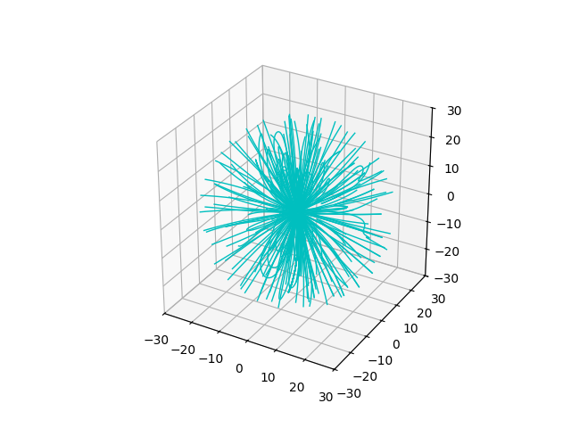
traces = tracer.trace_fbwd(launch_points=launch_points)

Plot traces using the plot_traces() utility function and adjust the field of view to be 30 Solar Radii in each direction.

ax = plt.figure().add_subplot(projection='3d')
plot_traces(traces, ax=ax, color='c')

FOV = 30  # Rsun
for dim in 'xyz':
    getattr(ax, f'set_{dim}lim3d')((-FOV, FOV))
ax.set_box_aspect([1, 1, 1])

plt.show()

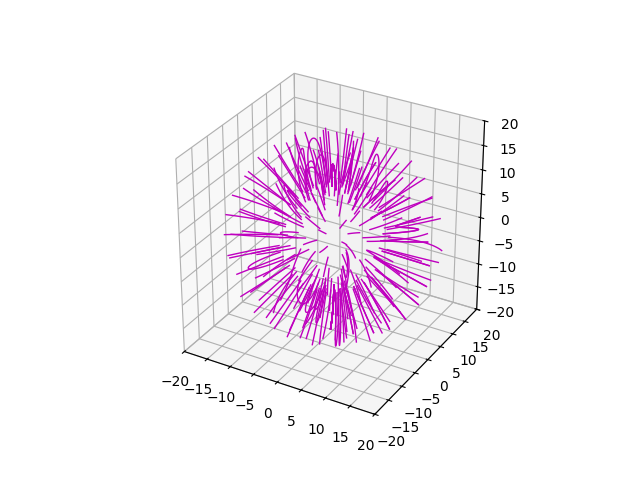
Now, adjust some of the mapfl parameters using the Tracer-as-dictionary pattern.

Attention

The base _Tracer class extends the MutableMapping interface, allowing users to interact with a tracer’s params property as if it were a dictionary.

tracer['domain_r_min_'] = 10    # Directly set the minimum radius parameter
tracer['domain_r_max_'] = 20    # Directly set the maximum radius parameter
traces = tracer.trace_fbwd(launch_points=launch_points)

ax = plt.figure().add_subplot(projection='3d')
plot_traces(traces, ax=ax, color='m')

FOV = 20  # Rsun
for dim in 'xyz':
    getattr(ax, f'set_{dim}lim3d')((-FOV, FOV))
ax.set_box_aspect([1, 1, 1])

plt.show()

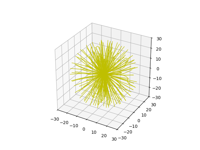
Similarly, one can use any of the native dict methods to manipulate the mapfl parameters, such as update().

tracer.update(domain_r_min_=1, domain_r_max_=30, cubic_=False, dsmult_=2)

Similarly, one can fetch views of the current parameters using the items(), keys(), and values() methods.

print("Tracer parameter keys:\n")
for key in tracer.keys():
    print(" - " + key)

Tracer parameter keys:

 - br
 - br_r
 - br_nr
 - br_t
 - br_nt
 - br_p
 - br_np
 - bt
 - bt_r
 - bt_nr
 - bt_t
 - bt_nt
 - bt_p
 - bt_np
 - bp
 - bp_r
 - bp_nr
 - bp_t
 - bp_nt
 - bp_p
 - bp_np
 - integrate_along_fl_
 - scalar_input_file_
 - verbose_
 - cubic_
 - trace_fwd_
 - trace_bwd_
 - trace_3d_
 - trace_slice_
 - compute_ch_map_
 - debug_level_
 - use_analytic_function_
 - function_params_file_
 - domain_r_min_
 - domain_r_max_
 - bfile_r_
 - bfile_t_
 - bfile_p_
 - ds_variable_
 - ds_over_rc_
 - ds_min_
 - ds_max_
 - ds_limit_by_local_mesh_
 - ds_local_mesh_factor_
 - ds_lmax_
 - set_ds_automatically_
 - dsmult_
 - rffile_
 - tffile_
 - pffile_
 - effile_
 - kffile_
 - qffile_
 - lffile_
 - rbfile_
 - tbfile_
 - pbfile_
 - ebfile_
 - kbfile_
 - qbfile_
 - lbfile_
 - new_r_mesh_
 - mesh_file_r_
 - nrss_
 - r0_
 - r1_
 - new_t_mesh_
 - mesh_file_t_
 - ntss_
 - t0_
 - t1_
 - new_p_mesh_
 - mesh_file_p_
 - npss_
 - p0_
 - p1_
 - volume3d_output_file_r_
 - volume3d_output_file_t_
 - volume3d_output_file_p_
 - slice_coords_are_xyz_
 - trace_slice_direction_is_along_b_
 - compute_q_on_slice_
 - q_increment_h_
 - slice_input_file_r_
 - slice_input_file_t_
 - slice_input_file_p_
 - trace_from_slice_forward_
 - slice_output_file_forward_r_
 - slice_output_file_forward_t_
 - slice_output_file_forward_p_
 - trace_from_slice_backward_
 - slice_output_file_backward_r_
 - slice_output_file_backward_t_
 - slice_output_file_backward_p_
 - slice_q_output_file_
 - slice_length_output_file_
 - ch_map_r_
 - ch_map_output_file_
 - compute_ch_map_3d_
 - ch_map_3d_output_file_
 - write_traces_to_hdf_
 - write_traces_root_
 - write_traces_as_xyz_

Once again, perform forward-backward tracing using the adjusted parameters.

traces = tracer.trace_fbwd(launch_points=launch_points)

ax = plt.figure().add_subplot(projection='3d')
plot_traces(traces, ax=ax, color='y')

FOV = 30  # Rsun
for dim in 'xyz':
    getattr(ax, f'set_{dim}lim3d')((-FOV, FOV))
ax.set_box_aspect([1, 1, 1])

plt.show()