Using Tracer Defaults

Perform simple tracing using the Tracer class.

This example demonstrates how to use the Tracer class to perform forward tracing of magnetic field lines from a set of default starting points.

Attention

The Tracer class enforces a singleton pattern to manage issues that arise from the underlying Fortran mapflpy_fortran object not being thread-safe. As a result, it is recommended to use the Tracer class in single-threaded contexts only viz. instantiating one instance of the class at a time.

import matplotlib.pyplot as plt

from mapflpy.tracer import Tracer
from mapflpy.utils import plot_traces
from mapflpy.data import fetch_cor_magfiles

Load in the magnetic field files

The fetch_cor_magfiles() function returns a tuple of file paths corresponding to the radial, theta, and phi components of the magnetic field data.

magnetic_field_files = fetch_cor_magfiles()

The Tracer class can be instantiated directly with the magnetic field file paths (along with any additional “mapfl params” as keyword arguments).

For now, the default mapfl configuration is used i.e. DEFAULT_PARAMS.

tracer = Tracer(*magnetic_field_files)

To illustrate the above-mentioned singleton behavior, if we attempt to create a second instance of the Tracer class while the first one is still in scope, we will encounter a RuntimeError.

try:
    tracer2 = Tracer()
except RuntimeError as e:
    print(e)

Multiple instances of Tracer within the same process are not supported. Use a single instance for tracing, or branch each Tracer into a subprocess.

The trace_fwd() method sets the tracing direction and performs forward tracing of magnetic field lines from a set of default launch points.

traces = tracer.trace_fwd()

The shape of the resulting traces geometry is an M x 3 x N array, where M is the field line length (i.e. the buffer_size), N is the number of launch points (here 128), and the second dimension corresponds to the radial-theta-phi coordinates.

The utility functions provided in utils are designed to work with this contiguous memory layout for efficient processing and visualization.

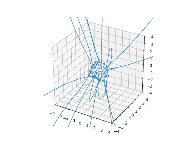
Plot traces using the plot_traces() utility function and adjust the field of view to be 4 Solar Radii in each direction

ax = plt.figure().add_subplot(projection='3d')
plot_traces(traces, ax=ax)

FOV = 4.0  # Rsun
for dim in 'xyz':
    getattr(ax, f'set_{dim}lim3d')((-FOV, FOV))
ax.set_box_aspect([1, 1, 1])

plt.show()