Filtering and Plotting Field Lines

Classify field line output and plot subsets of traces.

This example demonstrates how to use the get_fieldline_polarity() function to classify tracing output into the following categories:

• Open field lines connected to positive polarity regions at the domain inner boundary

• Open field lines connected to negative polarity regions at the domain inner boundary

• Closed field lines

• Disconnected field lines

• Field lines that failed to fully resolve within the tracing buffer size

These classifications can then be used to filter and visualize subsets of the traced field lines within distinct 3D plots.

import os

import numpy as np
from psi_io import np_interpolate_slice_from_hdf


import matplotlib
import matplotlib.pyplot as plt

from mapflpy.tracer import Tracer
from mapflpy.utils import plot_traces, get_fieldline_polarity, plot_sphere
from mapflpy.data import fetch_cor_magfiles
from mapflpy.globals import Polarity

Load in the magnetic field files and instantiate the Tracer

magnetic_field_files = fetch_cor_magfiles()
tracer = Tracer(*magnetic_field_files)

Here we create a set of 128 launch points arranged in a ring at r=15 Rsun and theta=pi/2 (equatorial plane).

r = 15.0  # Rs
t = np.pi / 2
p = np.linspace(0, 2 * np.pi, 128, endpoint=False)

rr, tt, pp = np.meshgrid(r, t, p, indexing='ij')
launch_points = np.column_stack((rr, tt, pp))[0,...]

traces = tracer.trace_fbwd(launch_points=launch_points)

The get_fieldline_polarity() function is used to classify the traces; the result of this operation yields an array of Polarity enum values (where the possible values are listed in the table below):

Enum Value	Integer Value	Description
R0_R1_NEG	-2	Open field line with negative polarity at inner boundary
R0_R0	-1	Closed field line
ERROR	0	Field line that failed to resolve within the buffer size
R1_R1	1	Disconnected field line
R0_R1_POS	2	Open field line with positive polarity at inner boundary

To properly classify the field lines, we need to provide the inner and outer radii of the domain and the filepath to the magnetic field file viz. used to determine the polarity at the inner boundary (here the radial component of the magnetic field).

Note

The atol (“absolute tolerance”) parameter is used to determine whether a field line footpoint is sufficiently close to the inner or outer boundary to be considered “anchored” there. This keyword argument is passed to isclose() when comparing the footpoint radius to the boundary radii.

polarity = get_fieldline_polarity(1,
                                  30,
                                  magnetic_field_files.br,
                                  traces,
                                  atol=1e-2)

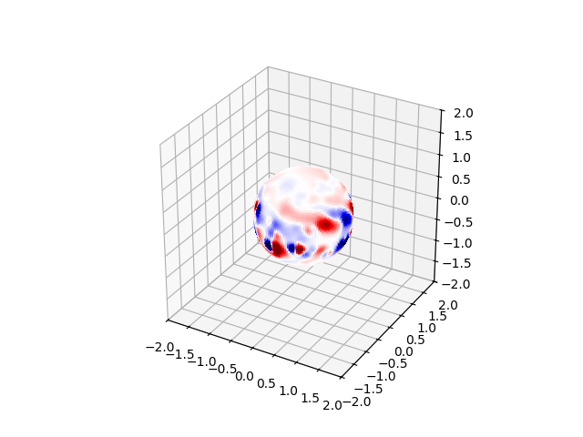
First, we plot the magnetic field sphere at 1 Rsun for context using the plot_sphere() utility function.

values, theta_scale, phi_scale = np_interpolate_slice_from_hdf(magnetic_field_files.br,
                                                           1.0, None, None,)
ax = plt.figure().add_subplot(projection='3d')
plot_sphere(values.T, 1.0, theta_scale, phi_scale, clim=(-10, 10), ax=ax)
FOV = 2  # Rsun
for dim in 'xyz':
    getattr(ax, f'set_{dim}lim3d')((-FOV, FOV))
ax.set_box_aspect([1, 1, 1])
plt.show()

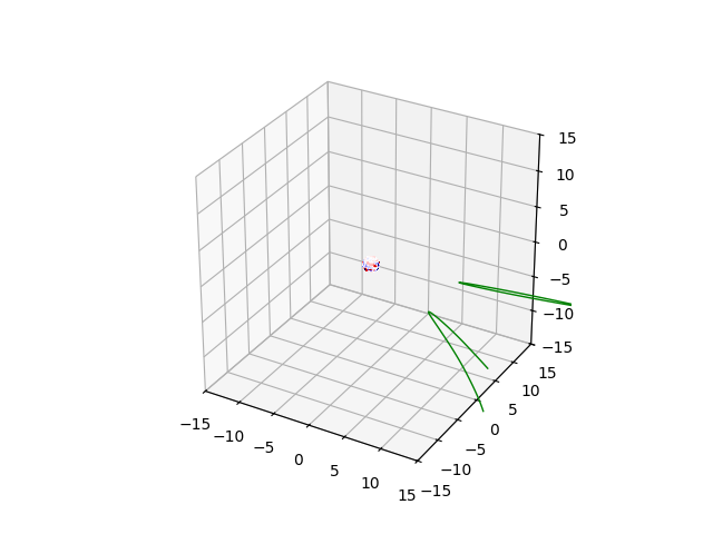
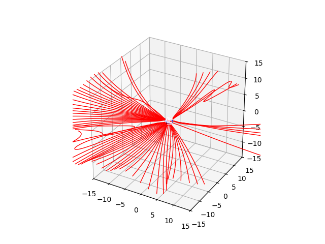
Next, we explicitly iterate over each polarity classification, filter the traces accordingly, and plot the resulting subset of field lines in a distinct 3D plot.

polarity_mapping = {
    Polarity.R0_R1_NEG: 'blue',
    Polarity.R0_R0: 'grey',
    Polarity.ERROR: 'black',
    Polarity.R1_R1: 'green',
    Polarity.R0_R1_POS: 'red',
}

for p, color in polarity_mapping.items():
    pmask = (polarity == p)
    if np.any(pmask):
        print(f'Polarity {p.name}: {np.sum(pmask)} field lines')
        ax = plt.figure().add_subplot(projection='3d')
        plot_traces(traces.geometry[...,pmask], ax=ax, color=color)
        plot_sphere(values.T, 1.0, theta_scale, phi_scale, clim=(-10, 10), ax=ax)
        FOV = 15  # Rsun
        for dim in 'xyz':
            getattr(ax, f'set_{dim}lim3d')((-FOV, FOV))
        ax.set_box_aspect([1, 1, 1])
        plt.show()

• 
• 
• 
• 

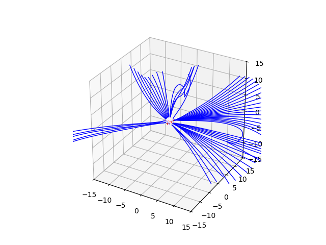
Polarity R0_R1_NEG: 53 field lines
Polarity R0_R0: 7 field lines
Polarity R1_R1: 2 field lines
Polarity R0_R1_POS: 66 field lines