Trace Forward & Backward

Perform combined forward-backward tracing of magnetic field lines.

This example demonstrates how to use the run_fwdbwd_tracing() function to trace magnetic field lines forward from a set of user-defined starting points.

import matplotlib.pyplot as plt
import matplotlib
import numpy as np

from mapflpy.scripts import run_fwdbwd_tracing
from mapflpy.utils import plot_traces, fetch_default_launch_points
from mapflpy.data import fetch_cor_magfiles

Load in the magnetic field files

The fetch_cor_magfiles() function returns a tuple of file paths corresponding to the radial, theta, and phi components of the magnetic field data.

magnetic_field_files = fetch_cor_magfiles()

Define launch points using the fibonacci lattice method.

Here we generate 256 launch points at a radius of 15 Rs.

launch_points = fetch_default_launch_points(256, r=15)

Run backward tracing using the defined launch points

traces = run_fwdbwd_tracing(*magnetic_field_files, launch_points=launch_points, context='fork')
print("Geometry shape:", traces.geometry.shape)

Geometry shape: (3999, 3, 256)

The shape of the resulting traces geometry is an M x 3 x N array, where M is the field line length (i.e. the buffer_size), N is the number of launch points (here 256), and the second dimension corresponds to the radial-theta-phi coordinates.

The utility functions provided in utils are designed to work with this contiguous memory layout for efficient processing and visualization.

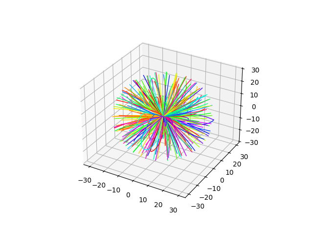
Plot traces using the plot_traces() utility function. Here we assign each trace a different color (using a HSV colormap) by passing in the colors keyword argument.

rsample = np.random.random_sample(size=launch_points.shape[-1])
colors = matplotlib.colormaps['hsv'](rsample)
ax = plt.figure().add_subplot(projection='3d')
plot_traces(traces, ax=ax, colors=colors)

plt.show()