Trace Backward

Perform backward tracing of magnetic field lines.

This example demonstrates how to use the run_backward_tracing() function to trace magnetic field lines forward from a set of user-defined starting points.

import numpy as np
import matplotlib.pyplot as plt

from mapflpy.scripts import run_backward_tracing
from mapflpy.utils import plot_traces
from mapflpy.data import fetch_cor_magfiles

Load in the magnetic field files

The fetch_cor_magfiles() function returns a tuple of file paths corresponding to the radial, theta, and phi components of the magnetic field data.

magnetic_field_files = fetch_cor_magfiles()

Define launch points in spherical coordinates (r, theta, phi); here we define a ring of points at r=30 Rs around the equatorial plane. The resultant array should have the shape (N, 3), where N is the number of launch points.

rvalues = 30
thetas = np.pi/2
phis = np.linspace(0, 2 * np.pi, 180)

rr, tt, pp = np.meshgrid(rvalues, thetas, phis, indexing='ij')
launch_points = np.column_stack((rr, tt, pp))[0,...]

Run backward tracing using the defined launch points

traces = run_backward_tracing(*magnetic_field_files,
                              launch_points=launch_points,
                              context=CONTEXT)
print("Geometry shape:", traces.geometry.shape)

Geometry shape: (2000, 3, 180)

The shape of the resulting traces geometry is an M x 3 x N array, where M is the field line length (i.e. the buffer_size), N is the number of launch points (here 180), and the second dimension corresponds to the radial-theta-phi coordinates.

The utility functions provided in utils are designed to work with this contiguous memory layout for efficient processing and visualization.

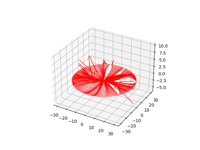
Plot traces using the plot_traces() utility function.

ax = plt.figure().add_subplot(projection='3d')
plot_traces(traces, ax=ax, color='red')
plt.show()