Mapping and Integrating Along Field Lines

This example demonstrates how to use the map_pt_forward() and map_pt_backward() functions to efficiently map large numbers of field lines on a grid from one spherical surface to another. These are based off a very general method for mapping field lines in parallel: map_field_lines_in_parallel().

This example also illustrates a related task: integrating scalar quantities along field lines. This can be used to compute scalar averages or other quantities. Weighting by the flux-tube area expansion is also possible. If no scalars are provided, the field-line length is provided by default.

import os
import tempfile

import numpy as np
from psi_io import wrhdf_3d, interpolate_positions_from_hdf
from psi_data import fetch_mas_data


import matplotlib
import matplotlib.pyplot as plt

from mapflpy.scripts import map_pt_forward, map_pt_backward

Load in the magnetic field and scalar field files used for this example. They are from a CORHEL-MAS thermodynamic MHD calculation for CR2282. Becuase they are not part of the standard datasets in mapflpy or psi-io (yet), we fetch them manually and place them in the default cache location.

files = fetch_mas_data(domains="cor", variables="br,bt,bp,t")
magnetic_field_files = files.cor_br, files.cor_bt, files.cor_bp
scalar_field_file = files.cor_t

  0%|                                              | 0.00/43.8M [00:00<?, ?B/s]
  1%|▌                                     | 623k/43.8M [00:00<00:07, 5.87MB/s]
  9%|███▏                                 | 3.81M/43.8M [00:00<00:01, 20.8MB/s]
 24%|████████▉                            | 10.6M/43.8M [00:00<00:00, 42.1MB/s]
 42%|███████████████▋                     | 18.5M/43.8M [00:00<00:00, 56.5MB/s]
 61%|██████████████████████▍              | 26.6M/43.8M [00:00<00:00, 65.1MB/s]
 79%|█████████████████████████████▏       | 34.5M/43.8M [00:00<00:00, 70.1MB/s]
 97%|████████████████████████████████████ | 42.6M/43.8M [00:00<00:00, 73.6MB/s]
  0%|                                              | 0.00/43.8M [00:00<?, ?B/s]
100%|██████████████████████████████████████| 43.8M/43.8M [00:00<00:00, 244GB/s]

First we compute a basic map by mapping field lines forward into the volume from a 2D grid on the surface and recording their endpoint locations. The mapping function accepts 1D arrays that specify the phi (longitude) and theta (co-latitude) grid in radians. It accepts the same mapfl options and keywords as the tracing routines (e.g. Tracer or run_forward_tracing()). Here the grid resolution is 1 degree, which should map relatively quickly on four processors (5-20 seconds).

# define the grid
radius = 1.0
t = np.linspace(0, np.pi, 181)
p = np.linspace(0, 2*np.pi, 361)

# compute the mapping
nproc = 4
mapping = map_pt_forward(*magnetic_field_files, p, t, radius=radius, nproc=nproc)

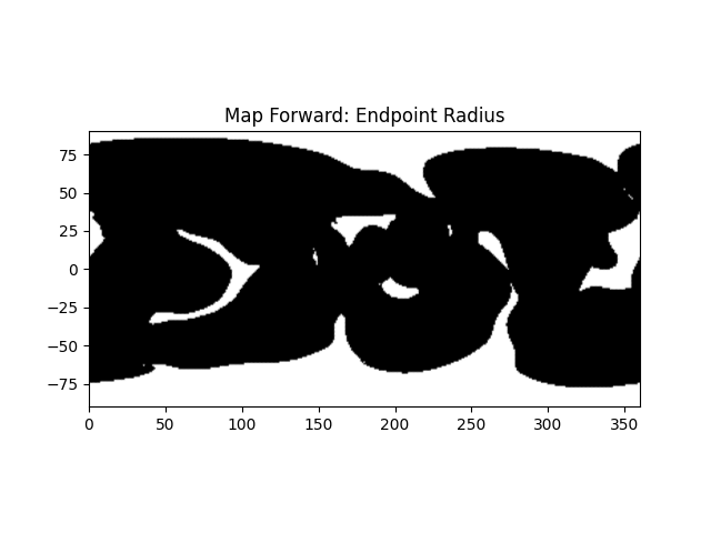
Next we can inspect the Mapping object, which contains the endpoint r, t, p values (2D arrays on the mapping grid in this case). Here we plot the endpoint radius, which indicates if a field line is open (30.0) or closed (1.0).

ax = plt.figure().add_subplot()
ax.pcolormesh(np.rad2deg(p), 90 - np.rad2deg(t), mapping.r,
              cmap='gray', shading='gouraud', clim=(1, 30))
ax.set_aspect("equal", adjustable="box")
ax.set_title('Map Forward: Endpoint Radius')
plt.show()

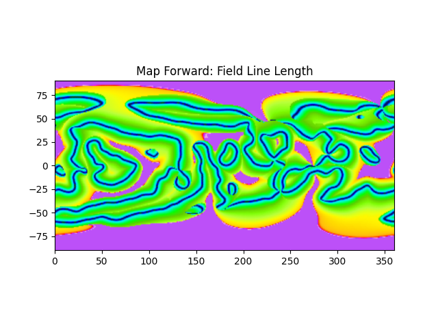
The mapping object also contains the field line length as the default integral field in units of solar radii. Here we plot it in log space to illustrate the dynamic range

ax = plt.figure().add_subplot()
ax.pcolormesh(np.rad2deg(p), 90 - np.rad2deg(t), np.log10(mapping.integral),
              cmap='gist_ncar', shading='gouraud', clim=(-2, 2))
ax.set_aspect("equal", adjustable="box")
ax.set_title('Map Forward: Field Line Length')
plt.show()

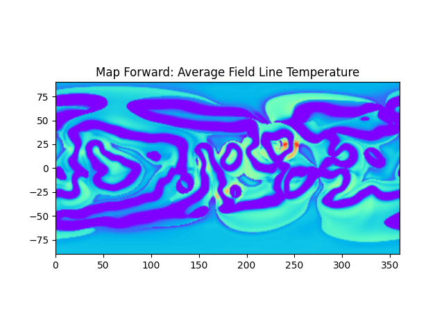
Instead of length we can integrate a 3D scalar along the field by setting mapfl accordingly. Currently, the scalar field must be passed as a path to a 3D HDF5 file. In this example we integrate temperature with a second mapping call. The average temperature along the magnetic field can be determined by dividing this integral by the length integral.

mapping2 = map_pt_forward(*magnetic_field_files, p, t, radius=radius, nproc=nproc,
                          integrate_along_fl_=True, scalar_input_file_=scalar_field_file)

# compute the average temperature in code units by dividing the two integrals
avg_t_mas = mapping2.integral/mapping.integral

# convert it to MK using the MAS normalizations
from psi_io.units import FN_T
import astropy.units as u

avg_t_mk = (avg_t_mas*FN_T).to(u.MK)
ax = plt.figure().add_subplot()
ax.pcolormesh(np.rad2deg(p), 90 - np.rad2deg(t), avg_t_mk.value,
              cmap='rainbow', shading='gouraud', clim=(0.5, 2.5))
ax.set_aspect("equal", adjustable="box")
ax.set_title('Map Forward: Average Field Line Temperature')
plt.show()

We can also weight the integrals by the relative flux-tube area by adding 1/B weighting. This allows one to construct other types of interesting scalar integrals. Here we use it to compute the relative field line volume: \(V_{FL} = \int_0^L A ds = A_0 B_0 \int_0^L \frac{1}{B}ds = |d\vec{A}\cdot \vec{B}_0| \int_0^L \frac{1}{B}ds= r^2d\Omega |B_r| \int_0^L \frac{1}{B}ds\) We do this by turning on weight_integral_by_area_ and passing a scalar field file that is equal to 1 at all points.

# create an interior p, t mesh (no poles) to make the area calculation simpler
p_i = 0.5*(p[1:] + p[0:-1])
t_i = 0.5*(t[1:] + t[0:-1])

# map foward from 1.0 to 2.0
domain_r_min = 1.0
domain_r_max = 2.0

# Build an all-ones scalar field for the 1/B area weighting. The value is
# constant, so a coarse (r, theta, phi) grid suffices — only the scales (which
# must bracket the traced volume) and the 3D-with-scales format matter. mapfl
# reads the scalar from disk, so we write it to a temporary file.
ones_r = np.array([domain_r_min, domain_r_max])
ones_t = np.array([0.0, np.pi])
ones_p = np.array([0.0, 2*np.pi])
ones_field = np.ones((ones_p.size, ones_t.size, ones_r.size))  # C-order: (nphi, ntheta, nr)
dummy_file = os.path.join(tempfile.gettempdir(), 'mapflpy_dummy_ones_3d.h5')
wrhdf_3d(dummy_file, ones_r, ones_t, ones_p, ones_field)
mappping_area_fwd = map_pt_forward(*magnetic_field_files, p_i, t_i, radius=domain_r_min, nproc=nproc,
                                   domain_r_min_=domain_r_min, domain_r_max_=domain_r_max,
                                   integrate_along_fl_=True, weight_integral_by_area_=True,
                                   scalar_input_file_=dummy_file)

# compute the area of each gridcell, adjusting the area factor at the pole for the half cell
# (use np.gradient with care, this is a simple example where it is fine).
dp = np.gradient(p_i)
dt = np.gradient(t_i)
cell_omega = np.einsum('i,j->ij', dt*np.sin(t_i), dp)

# get br at this surface by interpolating to the 2D grid of r, t, p positions
p2d, t2d = np.meshgrid(p_i, t_i)
ones2d = np.ones_like(p2d)
br_lower = interpolate_positions_from_hdf(files.cor_br, ones2d*domain_r_min, t2d, p2d)

# Compute the volume
vol_fwd = domain_r_min**2*cell_omega*np.abs(br_lower)*mappping_area_fwd.integral

ax = plt.figure().add_subplot()
ax.pcolormesh(np.rad2deg(p_i), 90 - np.rad2deg(t_i), np.log10(np.clip(vol_fwd, min=1e-5)),
              cmap='terrain', shading='gouraud', clim=(-5, -2))
ax.set_aspect("equal", adjustable="box")
ax.set_title('Map Forward: Field Line Volume [$R_S^3$]')
plt.show()

Lastly, we can confirm (for fun) that the volume calculation is correct by comparing the volume of the fowards and backwards maps to the analytic volume of a sphere.

# map backwards from radius=rmax
mapping_area_bwd = map_pt_backward(*magnetic_field_files, p_i, t_i, radius=domain_r_max, nproc=nproc,
                                   domain_r_min_=domain_r_min, domain_r_max_=domain_r_max,
                                   integrate_along_fl_=True, weight_integral_by_area_=True,
                                   scalar_input_file_=dummy_file)

br_upper = interpolate_positions_from_hdf(files.cor_br, ones2d*domain_r_max, t2d, p2d)
vol_bwd = domain_r_max**2*cell_omega*np.abs(br_upper)*mapping_area_bwd.integral

# the total volume should be the average of the two mapping's total volumes
# (all closed, open, and disconnected field lines only counted once)
vol_avg = 0.5*(np.sum(vol_fwd) + np.sum(vol_bwd))

# compare to the analytic volume
# NOTE: This agreement improves with more points in the mapping.
vol_analytic = 4./3.*np.pi*(domain_r_max**3 - domain_r_min**3)
print(f'### Volume check for {len(p_i)}x{len(t_i)} mappings from r = {domain_r_min} - {domain_r_max} Rs')
print(f'  Analytic Volume:     {vol_analytic:.4f}')
print(f'  Avg Total FL Volume: {vol_avg:.4f}')
print(f'  Percentage error:    {(vol_analytic - vol_avg)/vol_analytic*100:.2f} %')

### Volume check for 360x180 mappings from r = 1.0 - 2.0 Rs
  Analytic Volume:     29.3215
  Avg Total FL Volume: 29.3153
  Percentage error:    0.02 %