Loading and Plotting MHD Data

This example introduces the two steps needed to go from a PSI data file to a rendered scene:

1. Fetching a dataset — fetch_datasets() downloads (or retrieves from cache) a version-pinned HDF5 file from the PSI asset server and returns its local path.

2. Reading the data — read_hdf_by_index() loads the array values and the three coordinate grids \((r, \theta, \phi)\) from the file. Passing None for a dimension selects its full extent; passing an integer index fixes that dimension to a single grid point.

The dataset used here is the radial magnetic field \(B_r\) from a Thermo 2 steady-state coronal simulation for Carrington Rotation 2282 (CR 2282), covering the domain \(r \in [1,\,30]\,R_\odot\).

from psi_io import read_hdf_by_index
from pyvisual import Plot3d
from pyvisual.utils.data import fetch_datasets

Fetching a Dataset

fetch_datasets() accepts a domain identifier ('cor' for the coronal domain, 'hel' for heliospheric) and a variable name. It returns a namedtuple() whose fields are named "{domain}_{variable}". The first call downloads the file to the local cache; subsequent calls return the cached copy immediately without hitting the network.

datasets = fetch_datasets("cor", "br")
br_file = datasets.cor_br

Reading a 2-D Radial Slice

read_hdf_by_index() reads the HDF5 file and returns (data, r, t, p) — the scalar array followed by the three coordinate vectors. Index arguments control which portion of the grid is loaded:

• None — load the full extent of that dimension.

• An integer i — fix that dimension to the i-th grid point (1-based), collapsing it to a length-1 array.

Here the colatitude is fixed at index 71 (the equatorial plane, \(\theta_{71} \approx \pi/2\)), while \(r\) and \(\phi\) span their full extents. The result is a 2-D surface in the equatorial plane colored by \(B_r\).

data, r, t, p = read_hdf_by_index(br_file, None, 71, None)

plotter = Plot3d()
plotter.show_axes()
plotter.add_sun()
plotter.add_2d_slice(r, t, p, data, cmap='seismic', clim=(-1, 1),
                     show_scalar_bar=True)
plotter.show()

Static Scene

Interactive Scene

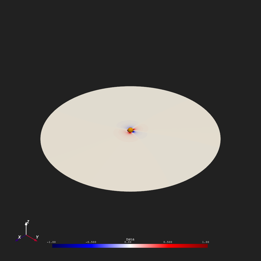
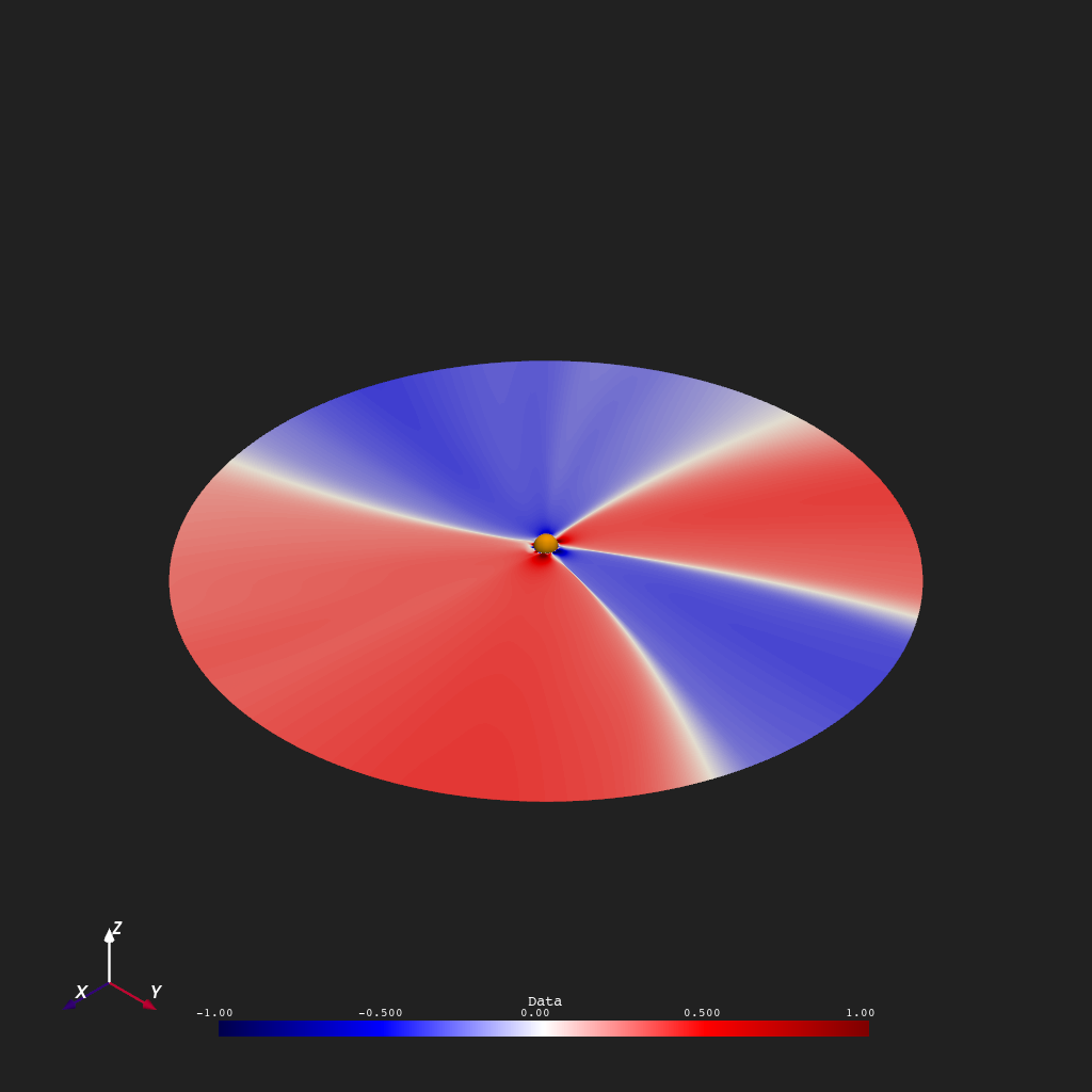
Scaling by \(r^2\)

The radial magnetic field falls off geometrically as \(1/r^2\) with distance. Multiplying by \(r^2\) removes this trend and reveals the longitudinal structure of open-field regions at all radii — a common diagnostic in solar wind modeling. Because r is a plain NumPy array, the scaling is a single element-wise operation before passing to the plotter.

plotter = Plot3d()
plotter.show_axes()
plotter.add_sun()
plotter.add_2d_slice(r, t, p, data * r ** 2, cmap='seismic', clim=(-1, 1),
                     show_scalar_bar=True)
plotter.show()

Static Scene

Interactive Scene