Constructing a SphericalMesh

This example demonstrates the three ways to initialise a SphericalMesh:

1. From an HDF file path — pass the path directly; the constructor calls read_hdf_by_index() internally. Additional positional arguments after the path are forwarded as index arguments to the file reader.

2. From data arrays — read the file manually with read_hdf_by_index(), then pass the coordinate arrays and data to the constructor.

3. From an existing SphericalMesh — pass another mesh instance to produce a shallow copy.

All three routes produce an equivalent mesh; the choice depends on how much control over the read step you need. Real coronal magnetic field data \(B_r\) from a PSI Thermo 2 run for Carrington Rotation 2282 (CR 2282) is used throughout.

from psi_io import read_hdf_by_index
from pyvisual import Plot3d
from pyvisual.core.mesh3d import SphericalMesh
from pyvisual.utils.data import fetch_datasets

br_file = fetch_datasets("cor", "br").cor_br

From an HDF File Path

Passing a file path as the first argument triggers the file-path dispatch path: the constructor calls read_hdf_by_index() on the path, loading both the scalar data and the three coordinate grids. Positional arguments after the path are forwarded to read_hdf_by_index() as index arguments, controlling which portion of the grid is loaded (see the function documentation for details).

Here no index arguments are supplied, so the full 3-D coronal domain is loaded (\(r \times \theta \times \phi\)).

mesh_from_path = SphericalMesh(br_file)

print(f"dimensions : {mesh_from_path.dimensions}")
print(f"r range    : [{mesh_from_path.r.min():.2f}, {mesh_from_path.r.max():.2f}] R_sun")
print(f"t range    : [{mesh_from_path.t.min():.4f}, {mesh_from_path.t.max():.4f}] rad")
print(f"p range    : [{mesh_from_path.p.min():.4f}, {mesh_from_path.p.max():.4f}] rad")
print(f"data range : [{mesh_from_path.data.min():.4f}, {mesh_from_path.data.max():.4f}] MAS Units")

dimensions : (255, 142, 299)
r range    : [1.00, 30.42] R_sun
t range    : [0.0000, 3.1416] rad
p range    : [0.0000, 6.2832] rad
data range : [-47.3395, 47.9679] MAS Units

From Data Arrays

When you need to pre-process the arrays before constructing the mesh — for example to apply a coordinate transform or inspect the raw values — call read_hdf_by_index() yourself and pass the results directly to the constructor. The coordinate arrays go in as the first three positional arguments (r, t, p); the scalar values are supplied via the data keyword.

data, r, t, p = read_hdf_by_index(br_file)

mesh_from_arrays = SphericalMesh(r, t, p, data=data, dataid='Br')

# Dimensions and data range are identical to the file-path route.
print(f"dimensions match : {mesh_from_arrays.dimensions == mesh_from_path.dimensions}")
print(f"data allclose    : {(mesh_from_arrays.data == mesh_from_path.data).all()}")

dimensions match : True
data allclose    : True

From an Existing SphericalMesh

Passing an existing SphericalMesh (or any pyvista.DataSet) produces a shallow copy — both objects share the same underlying data buffers. Pass deep=True for an independent copy.

mesh_from_mesh = SphericalMesh(mesh_from_path)

print(f"dimensions match : {mesh_from_mesh.dimensions == mesh_from_path.dimensions}")

dimensions match : True

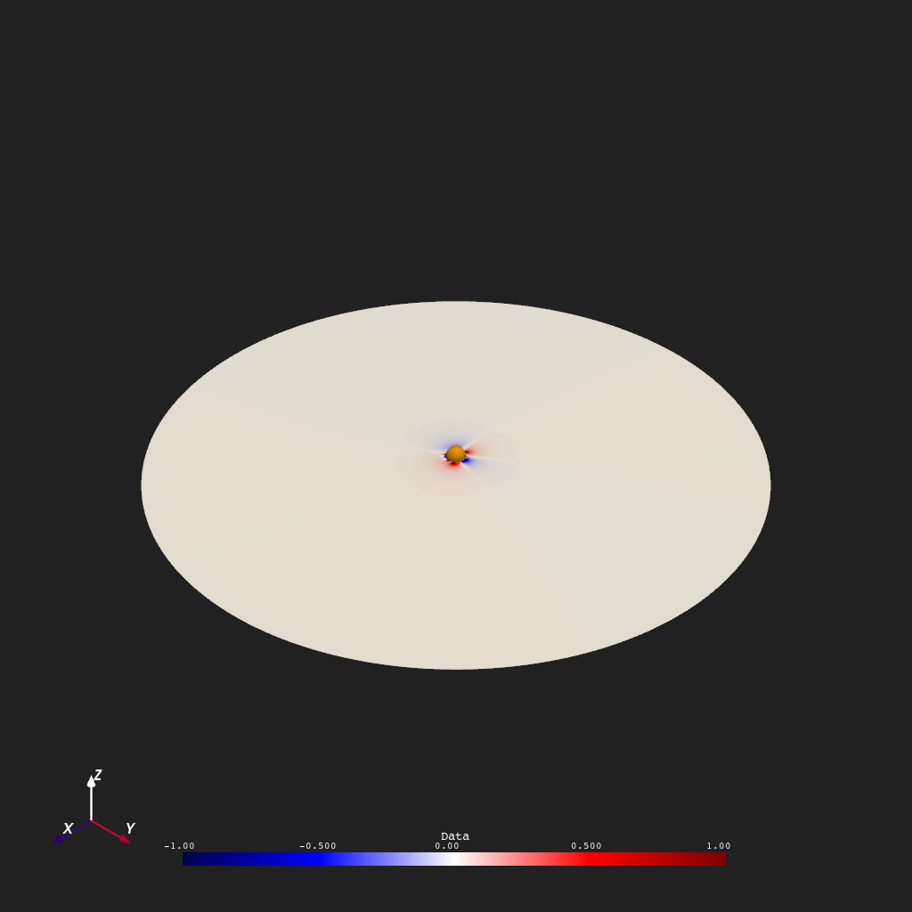
Visualising the Mesh

All three meshes are equivalent. Here the equatorial plane is extracted by slicing the theta axis (\(\theta_{71} \approx \pi/2\)) and rendered as a 2-D surface colored by \(B_r\). The MESH_FRAME tag stored in user_dict tells Plot3d to convert spherical coordinates to Cartesian automatically before rendering.

equatorial = mesh_from_path[:, 71, :]

plotter = Plot3d()
plotter.show_axes()
plotter.add_sun()
plotter.add_mesh(equatorial, cmap='seismic', clim=(-1, 1), show_scalar_bar=True)
plotter.show()

Static Scene

Interactive Scene