Arithmetic and NumPy Ufunc Support

CartesianMesh (and SphericalMesh) inherit a full arithmetic suite from _BaseFrameMesh. Standard Python operators (+, -, *, /, **, etc.) and NumPy ufuncs such as numpy.log10 and numpy.sqrt operate element-wise on the active scalar field and return a new mesh of the same type with the result as the active scalar. The coordinate arrays are never modified — only the data changes.

import numpy as np
from pyvisual import Plot3d
from pyvisual.core.mesh3d import CartesianMesh

Build a Mesh

Construct a CartesianMesh over a regular Cartesian grid. The scalar data is the Euclidean distance \(r = \sqrt{x^2 + y^2 + z^2}\) from the origin, providing a smooth, sign-definite field on which to demonstrate arithmetic operations.

x = np.linspace(-5, 5, 20)
y = np.linspace(-5, 5, 20)
z = np.linspace(-5, 5, 20)
X, Y, Z = np.meshgrid(x, y, z, indexing='ij')
dist = np.sqrt(X ** 2 + Y ** 2 + Z ** 2)

mesh = CartesianMesh(X, Y, Z, data=dist, dataid='r')
print(f"data range : [{mesh.data.min():.2f}, {mesh.data.max():.2f}]")

data range : [0.46, 8.66]

Scalar Arithmetic

Standard Python arithmetic operators act element-wise on the active scalar field and return a new CartesianMesh — the point coordinates are untouched. Here we subtract the field minimum to shift the distribution to zero, then divide by the resulting maximum to normalise to the range \([0, 1]\).

mesh_shifted = mesh - mesh.data.min()
mesh_norm = mesh_shifted / mesh_shifted.data.max()
print(f"normalised range : [{mesh_norm.data.min():.2f}, {mesh_norm.data.max():.2f}]")

plotter = Plot3d()
plotter.show_axes()
plotter.add_sun()
plotter.add_mesh(mesh_norm, cmap='plasma', clim=(0, 1), opacity=0.3, show_scalar_bar=False)
plotter.show()

Static Scene

Interactive Scene

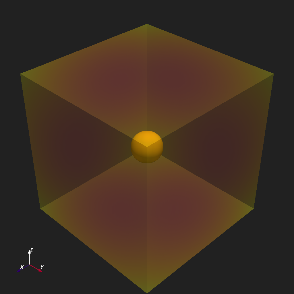
normalised range : [0.00, 1.00]

NumPy Ufunc: np.log10

The __array_ufunc__() hook lets any single-output NumPy ufunc act directly on the mesh. numpy.log10 applied to the normalised distance converts the field to a logarithmic scale that compresses the large dynamic range near the outer boundary and reveals structure close to the origin. Points at or below zero (here, the grid corner where \(r = 0\)) are masked by the log.

mesh_log = np.log10(mesh_norm + 1e-6)
print(f"log10 range : [{mesh_log.data.min():.2f}, {mesh_log.data.max():.2f}]")

plotter = Plot3d()
plotter.show_axes()
plotter.add_sun()
plotter.add_mesh(mesh_log, cmap='rainbow', clim=(-3, 0), opacity=0.3, show_scalar_bar=False)
plotter.show()

Static Scene

Interactive Scene

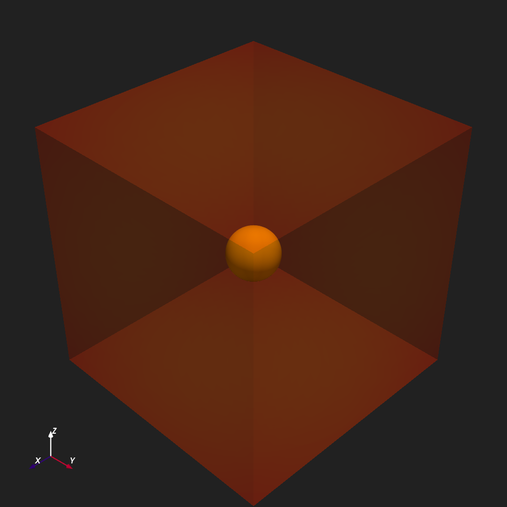
log10 range : [-6.00, 0.00]