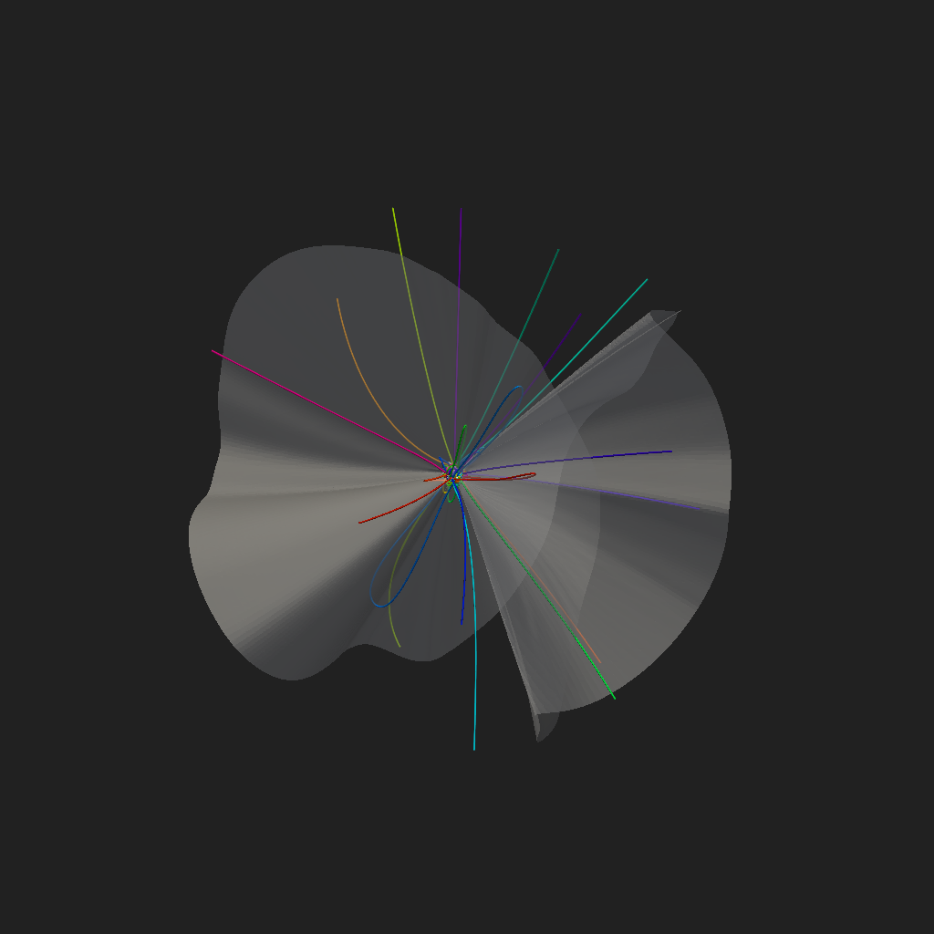
Combining Slices, Contours, and Fieldlines

This example demonstrates a complete coronal scene that combines a 2-D radial shell (coronal hole map), an isosurface contour of the radial magnetic field \(B_r\), and a bundle of magnetic fieldlines colored by random hue — illustrating how GridMeshMixin and StackMeshMixin methods can be layered in a single Plot3d scene.

Static Scene

Interactive Scene

from __future__ import annotations

import numpy as np
from mapflpy.tracer import Tracer
from psi_data import fetch_mas_data, fetch_mas_quantities
from psi_io import read_hdf_data

from pyvisual import Plot3d

data_files = fetch_mas_data(domains="cor", variables=["br", "bt", "bp"])
chmap_files = fetch_mas_quantities(quantities="ch_pm")

tracer = Tracer(data_files.cor_br, data_files.cor_bt, data_files.cor_bp)
fieldlines = tracer.trace_fwd(r=1.0, n=256)


chmap, *chmap_scales = read_hdf_data(chmap_files.ch_pm)
br, *br_scales = read_hdf_data(data_files.cor_br)

plotter = Plot3d()

plotter.add_longitudinal_lines()
plotter.add_latitudinal_lines()

plotter.add_2d_slice(1, *reversed(chmap_scales), chmap.T, cmap="seismic", show_scalar_bar=False)
plotter.add_contour(*br_scales, br, opacity=0.5, color="white", show_scalar_bar=False)
plotter.add_fieldlines(
    *np.moveaxis(fieldlines.geometry, 1, 0),
    line_width=2,
    coloring="random",
    cmap="hsv",
    name="fieldlines",
)
plotter.show()