Note
Go to the end to download the full example code.
MHDweb Integration Part II#
This is the second of a two-part series. MHDweb Integration Part I queried the MHDweb REST API to download coronal and heliospheric \((B_r, B_\theta, B_\phi)\) field files and the Solar Orbiter spacecraft connectivity mapping; this example loads those outputs and produces four visualizations:
A radially scaled overview of \(B_r\) in both model domains.
A static scene of the coronal \(B_r\) slice with spacecraft positions, ballistically mapped positions, and backward-traced coronal connectivity.
An animation of inter-domain and spacecraft mapping traces from a fixed wide-angle heliospheric perspective.
A close-up coronal animation whose camera follows each spacecraft’s longitude through the sequence.
Magnetic connectivity is computed in two ways:
Spacecraft mapping —
TracerMPtraces backward from the ballistically mapped positions at \(r_1 \approx 30\,R_\odot\) through the coronal domain. The spacecraft position is then prepended to form a continuous path from the heliosphere to the solar surface.Inter-domain tracing —
_inter_domain_tracing()launches field-line integration from the spacecraft positions directly, crossing the coronal–heliospheric domain boundary to produce end-to-end connectivity from the spacecraft to \(r_0 = 1\,R_\odot\).
See also
- MHDweb Integration Part I
Part I — queries MHDweb, downloads field files, and saves the spacecraft mapping table.
- Plotting Magnetic Fieldlines
Introduction to fieldline rendering with
add_fieldlines().
from __future__ import annotations

import os
from contextlib import ExitStack
from math import pi
from pathlib import Path
from zipfile import ZipFile

import astropy.units as u
import numpy as np
from astropy.table import QTable
from mapflpy.scripts import _inter_domain_tracing
from mapflpy.tracer import TracerMP
from mapflpy.utils import combine_and_pad_fieldlines
from sunpy.sun.constants import sidereal_rotation_rate

from pyvisual import Plot3d, SphericalMesh
Extract and Load Field Data#
The ZIP archives downloaded in Part I are extracted to their respective
directories. SphericalMesh loads each
br002.h5 file directly.
OUTPUT_DIR = Path(os.environ.get("STATIC_ASSETS", "")).resolve()
COR_OUTPUT_DIR = OUTPUT_DIR / "cor_mag_field"
HEL_OUTPUT_DIR = OUTPUT_DIR / "hel_mag_field"

print("Extracting coronal magnetic field files...")         # noqa: T201
with ZipFile(COR_OUTPUT_DIR / "cor_mag_field.zip") as cor_zip:
    print(f"cor_mag_field.zip namelist: {cor_zip.namelist()}")              # noqa: T201
    cor_zip.extractall(path=COR_OUTPUT_DIR)
print("Extracting heliospheric magnetic field files...")            # noqa: T201
with ZipFile(HEL_OUTPUT_DIR / "hel_mag_field.zip") as hel_zip:
    print(f"hel_mag_field.zip namelist: {hel_zip.namelist()}")              # noqa: T201
    hel_zip.extractall(path=OUTPUT_DIR / "hel_mag_field")

cor_br_mesh = SphericalMesh(COR_OUTPUT_DIR / "br002.h5")
hel_br_mesh = SphericalMesh(HEL_OUTPUT_DIR / "br002.h5")
Extracting coronal magnetic field files...
cor_mag_field.zip namelist: ['br002.h5', 'bt002.h5', 'bp002.h5']
Extracting heliospheric magnetic field files...
hel_mag_field.zip namelist: ['br002.h5', 'bt002.h5', 'bp002.h5']
Parse the Spacecraft Mapping Table#
The ECSV file written in Part I is read into an
astropy.table.QTable, which preserves column units (distances in
\(R_\odot\), angles in radians).
The three position arrays — each of shape \((3, N)\) in \((r, \theta, \phi)\) order — correspond to the three legs of the spacecraft connectivity chain returned by the MHDweb spacecraft-mapping endpoint:
spacecraft_positions— actual spacecraft location.balmapped_positions— position ballistically mapped to the outer coronal boundary \(r_1 \approx 30\,R_\odot\).traced_positions— magnetic footpoint at the inner boundary \(r_0 = 1\,R_\odot\).
spacecraft_mapping = QTable.read(OUTPUT_DIR / "spacecraft_mapping.ecsv", format="ascii.ecsv")

spacecraft_positions = np.stack(tuple(spacecraft_mapping[f"sc_pos_{dim}"].value for dim in "rtp"))
balmapped_positions = np.stack(tuple(spacecraft_mapping[f"r1_pos_{dim}"].value for dim in "rtp"))
traced_positions = np.stack(tuple(spacecraft_mapping[f"r0_pos_{dim}"].value for dim in "rtp"))
To properly visualize the ballistic mappings, we need to construct a continuous path from the spacecraft position through the heliosphere to the coronal footpoint.
For each time step, a radial path is constructed from 50 linearly spaced radial
positions (beginning from the spacecraft position and ending at \(30\,R_\odot\)).
The time shift for each radial position is computed based on the in situ flow speed, and the
corresponding longitudinal shift is calculated using
sunpy’s sidereal_rotation_rate.
balmapping_radial_path = np.linspace(spacecraft_mapping["sc_pos_r"].value, 30, 50) * u.R_sun
time_shift = (spacecraft_mapping["sc_pos_r"] - balmapping_radial_path) / (
    spacecraft_mapping["flow_speed"]
)
longitudinal_shift = time_shift * sidereal_rotation_rate
balmapping_longitudinal_path = (
    (spacecraft_mapping["sc_pos_p"] + longitudinal_shift) % (360 * u.deg)
).to(u.rad)

ballistic_mapping_trajectory = np.stack(
    (
            balmapping_radial_path.value,
            np.full_like(balmapping_radial_path.value, spacecraft_positions[1]),
            balmapping_longitudinal_path.value,
    ),
    axis=1,
)
Trace Magnetic Connectivity#
TracerMP is a multiprocessing-capable tracer that
must be used as a context manager; contextlib.ExitStack manages
two tracer contexts simultaneously so that both are cleanly shut down even
if an exception occurs.
Spacecraft mapping traces — backward integration from
balmapped_positions (at \(r_1\)) through the coronal domain. The
spacecraft positions are prepended along axis 0 so the resulting array
represents the complete path from the heliosphere through to the coronal
footpoint.
Inter-domain traces — _inter_domain_tracing()
launches from the actual spacecraft positions and integrates through both
the heliospheric and coronal domains, crossing the domain boundary
automatically. combine_and_pad_fieldlines() merges
the per-domain segments into a single NaN-padded array suitable for
add_splines().
with ExitStack() as cstack:
    cor_tracer = cstack.enter_context(
            TracerMP(*[COR_OUTPUT_DIR / f"b{dim}002.h5" for dim in "rtp"], context="fork")
    )
    hel_tracer = cstack.enter_context(
            TracerMP(*[HEL_OUTPUT_DIR / f"b{dim}002.h5" for dim in "rtp"], context="fork")
    )

    spacecraft_mapping_traces = cor_tracer.trace_bwd(launch_points=balmapped_positions)
    spacecraft_mapping_traces = np.concatenate(
            (ballistic_mapping_trajectory, spacecraft_mapping_traces.geometry)
    )

    inter_domain_traces, *_ = _inter_domain_tracing(
            cor_tracer, hel_tracer, launch_points=spacecraft_positions
    )
    inter_domain_traces = combine_and_pad_fieldlines(inter_domain_traces)

common_kwargs = {"cmap": "seismic", "clim": 10, "show_scalar_bar": False}
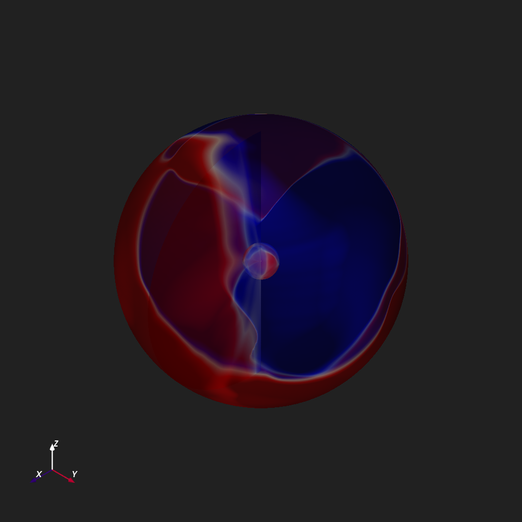
Two-Domain \(B_r\) Overview#
Both coronal and heliospheric \(B_r\) meshes are rendered in a single scene to provide context for the connectivity visualizations that follow.
plotter = Plot3d()
plotter.add_axes()
plotter.add_mesh(cor_br_mesh.radially_scale(), opacity=0.8, **common_kwargs)
plotter.add_mesh(hel_br_mesh.radially_scale(), opacity=0.6, **common_kwargs)
plotter.show()
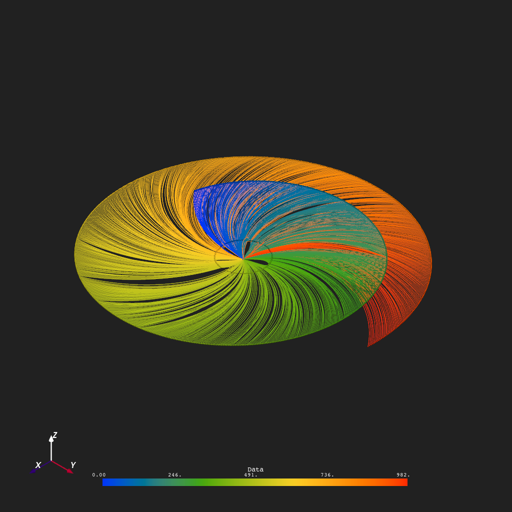
Spacecraft Connectivity in the Corona#
Spacecraft positions (colored by time index) and
ballistically mapped positions are shown as point clouds; the backward
traces connecting them through the coronal domain are rendered as splines.
numpy.moveaxis() transposes the geometry array from
\((M, 3, N)\) to \((3, M, N)\) for unpacking into
add_splines().
plotter = Plot3d()
plotter.add_axes()
plotter.add_mesh(cor_br_mesh.slice(normal="x", origin=(1, 0, 0)), opacity=0.8, **common_kwargs)
plotter.add_points(*spacecraft_positions, np.arange(len(spacecraft_mapping)), point_size=3)
plotter.add_points(*balmapped_positions, np.arange(len(spacecraft_mapping)), point_size=3)
plotter.add_splines(
    *np.moveaxis(spacecraft_mapping_traces, 1, 0), np.arange(len(spacecraft_mapping))
)
plotter.show()
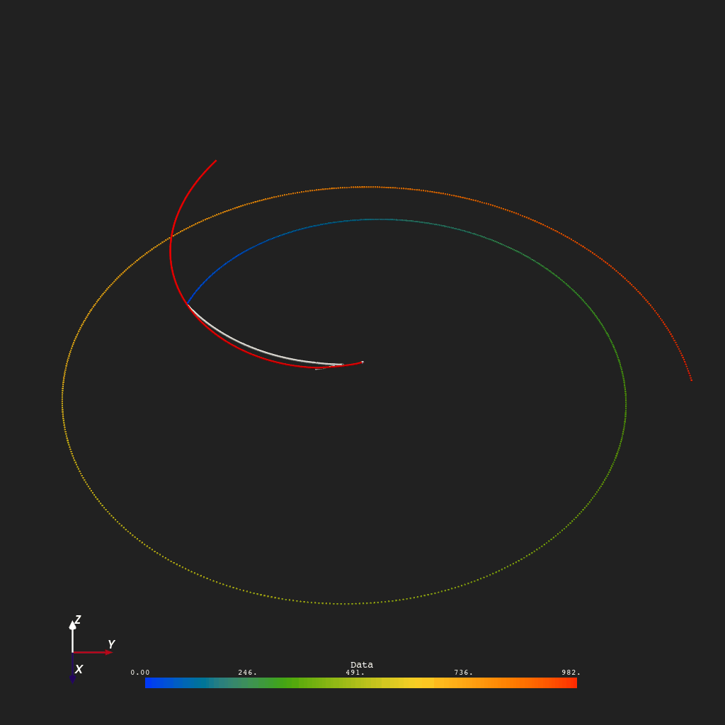
Animate Spacecraft Mapping in the Heliosphere#
A fixed wide-field observer at \((r, \theta, \phi) = (400\,R_\odot,\;\pi/4,\;0)\) with a \(200^\circ\) field of view frames the entire heliospheric domain. Each frame advances one time step, drawing the spacecraft mapping trace (white) and inter-domain trace (red) in a rolling buffer of five named actors so the scene never accumulates more than five trace pairs.
plotter = Plot3d()
plotter.add_axes()
plotter.add_points(*spacecraft_positions, np.arange(len(spacecraft_mapping)), point_size=3)
plotter.add_mesh(cor_br_mesh[1, ...], **common_kwargs)
plotter.observer_position = 400, pi / 4, 0
plotter.observer_fov_view = 200
plotter.open_gif(OUTPUT_DIR / "spacecraft_mapping_heliosphere.gif", fps=40)
for i, (scmap_trace, interdomain_trace) in enumerate(
    zip(spacecraft_mapping_traces.T, inter_domain_traces.T, strict=True)
):
    plotter.add_spline(*scmap_trace, name=f"scmap_trace_{i % 5}", color="white", line_width=3)
    plotter.add_spline(
            *interdomain_trace, name=f"interdomain_trace_{i % 5}", color="red", line_width=3
    )
    plotter.write_frame()
plotter.close()
/Users/rdavidson/MHDweb/pyvisual/pyvisual/utils/geometry.py:968: UserWarning: 'where' used without 'out', expect unitialized memory in output. If this is intentional, use out=None.
  np.where(mask, np.pi - np.arcsin(2 - ratio, where=mask), np.arcsin(ratio, where=~mask))
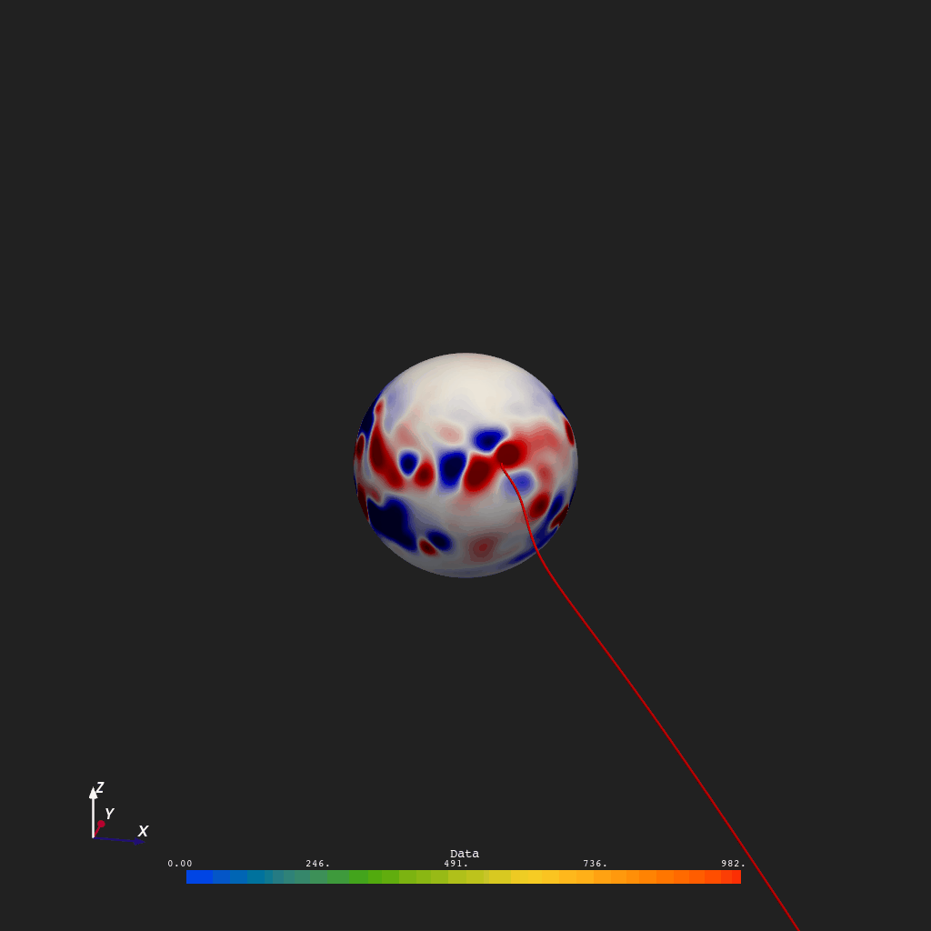
Animate Spacecraft Mapping in the Corona#
The same traces are re-animated from a close-up coronal perspective. The observer is placed at \(r = 15\,R_\odot\) near the ecliptic (\(\theta = 3\pi/8\)) and its longitude tracks each spacecraft position plus a \(\pi/6\) offset, keeping the active trace near the center of the \(4^\circ\) field of view as the sequence progresses.
plotter = Plot3d()
plotter.add_axes()
plotter.add_points(*spacecraft_positions, np.arange(len(spacecraft_mapping)), point_size=3)
plotter.add_mesh(cor_br_mesh[1, ...], **common_kwargs)
plotter.open_gif(OUTPUT_DIR / "spacecraft_mapping_corona.gif", fps=40)
for i, (scmap_trace, interdomain_trace) in enumerate(
    zip(spacecraft_mapping_traces.T, inter_domain_traces.T, strict=True)
):
    plotter.observer_position = 15, 3 * pi / 8, spacecraft_positions[2, i] + pi / 6
    plotter.observer_fov_view = 4
    plotter.add_spline(*scmap_trace, name=f"scmap_trace_{i % 5}", color="white", line_width=3)
    plotter.add_spline(
            *interdomain_trace, name=f"interdomain_trace_{i % 5}", color="red", line_width=3
    )
    plotter.write_frame()
plotter.close()
Total running time of the script: (3 minutes 10.698 seconds)