Isosurface Contours

This example demonstrates add_contour() — the method for extracting and rendering an isosurface from a 3-D spherical scalar field.

Internally, add_contour() builds a SphericalMesh from the supplied coordinate arrays and scalar data, then calls contour() to extract the isosurface at the requested value before converting the result to Cartesian coordinates for rendering. Multiple isovalues can be passed as an array.

import numpy as np
from pyvisual import Plot3d

Magnetic Current Sheet

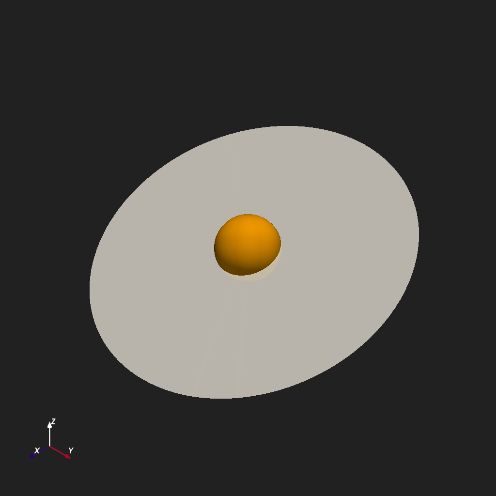
The heliospheric current sheet (HCS) is the surface in the corona and heliosphere where the radial magnetic field \(B_r\) reverses polarity. In a pure dipole, this surface is the flat equatorial plane; in a tilted or warped dipole, it becomes the “ballerina skirt” structure traced by spacecraft in situ measurements.

Below, a synthetic tilted-dipole field is constructed by adding a small azimuthal perturbation to a pure dipole \(B_r \propto \cos\theta\). The \(B_r = 0\) isosurface then reveals the wavy current sheet.

r = np.linspace(1, 5, 30)
t = np.linspace(0, np.pi, 60)
p = np.linspace(0, 2 * np.pi, 120)
R, T, P = np.meshgrid(r, t, p, indexing='ij')

# Tilted dipole: pure cos(theta) plus a longitude-dependent tilt
Br = np.cos(T) + 0.4 * np.cos(P) * np.sin(T)

plotter = Plot3d()
plotter.show_axes()
plotter.add_sun()
plotter.add_contour(r, t, p, Br, isovalue=0, color='white', opacity=0.8)
plotter.show()

Static Scene

Interactive Scene

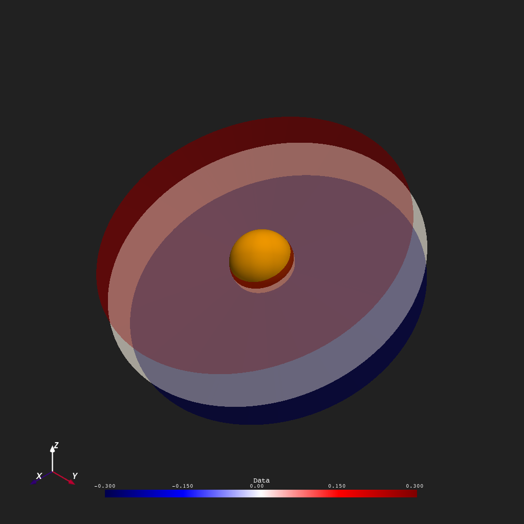
Multiple Isovalues

Passing an array to isovalue extracts several isosurfaces in a single call. Here three nested surfaces are extracted at \(B_r \in \{-0.3, 0, +0.3\}\), colored by value to distinguish the positive-polarity, neutral, and negative-polarity boundaries.

plotter = Plot3d()
plotter.show_axes()
plotter.add_sun()
plotter.add_contour(r, t, p, Br, isovalue=[-0.3, 0.0, 0.3],
                    cmap='seismic', clim=(-0.3, 0.3), opacity=0.7)
plotter.show()

Static Scene

Interactive Scene

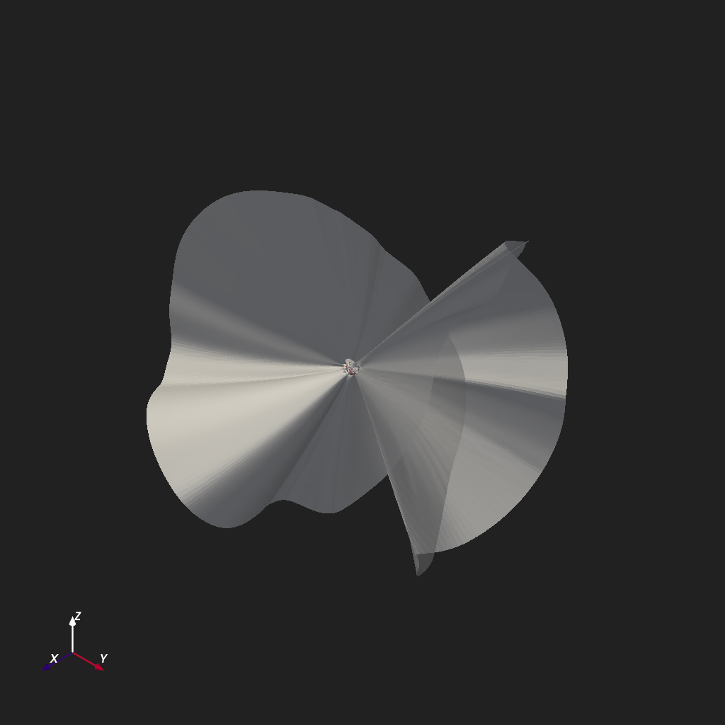
Using MAS Data

To demonstrate this contouring method on \(B_r\) data from a steady-state Thermodynamic MAS coronal model, we can load in the data using read_hdf_data().

from psi_io import read_hdf_data
from pyvisual.utils.data import fetch_datasets

br_file = fetch_datasets("cor", "br").cor_br
br, r, t, p = read_hdf_data(br_file)

plotter = Plot3d()
plotter.show_axes()
plotter.add_2d_slice(r[1], t, p, br[...,1], cmap='seismic', clim=(-30, 30),
                     show_scalar_bar=False)
plotter.add_contour(r, t, p, br, isovalue=0, color='white', opacity=0.9)
plotter.show()

Static Scene

Interactive Scene