2-D Surface Slices

This example demonstrates add_2d_slice() — the method for rendering a 2-D surface at a fixed spherical coordinate.

Exactly one of r, t, p must be a size-1 array, pinning that coordinate. The other two axes define the surface grid. The fixed axis is inferred automatically, and the result is rendered as a quad-faced surface colored by the supplied data array.

The three fundamental 2-D slice orientations in spherical geometry are the radial shell (fixed \(r\)), the theta cut (fixed \(\theta\)), and the phi cut (fixed \(\phi\)). Each is produced here by passing a single integer index for the pinned dimension to read_hdf_by_index(); None selects the full extent of the remaining two axes.

from psi_io import read_hdf_by_index
from pyvisual import Plot3d
from pyvisual.utils.data import fetch_datasets

Radial Shell

Fix \(r = r_1 \approx 1\,R_\odot\) and vary both \(\theta\) and \(\phi\) over their full extents. The resulting surface is a spherical shell at the inner coronal boundary, colored by the radial magnetic field \(B_r\) — the photospheric boundary condition for the MAS coronal model.

br_file = fetch_datasets("cor", "br").cor_br
data, r, t, p = read_hdf_by_index(br_file, 1, None, None)

plotter = Plot3d()
plotter.show_axes()
plotter.add_sun()
plotter.add_2d_slice(r, t, p, data, cmap='seismic', clim=(-30, 30),
                     show_scalar_bar=False)
plotter.show()

Static Scene

Interactive Scene

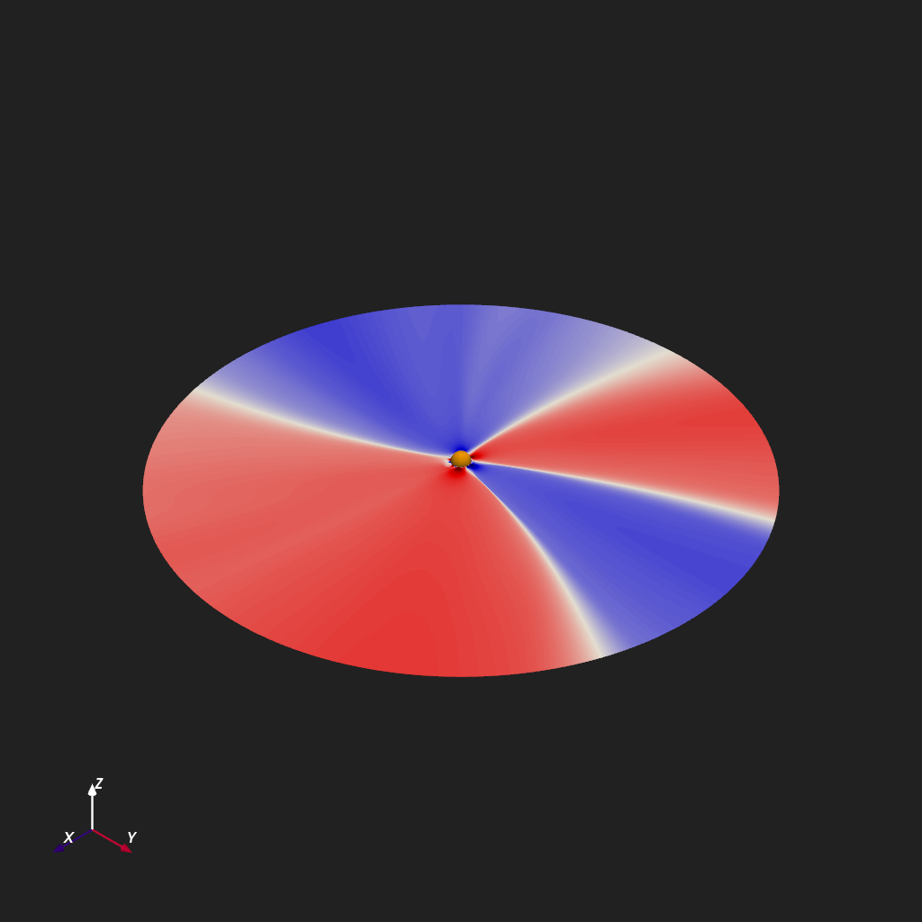
Theta Cut (Equatorial Plane)

Fix the colatitude at the equatorial plane (\(\theta = \theta_{71} \approx \pi/2\)) and vary both \(r\) and \(\phi\) over their full extents. The surface is colored by the signed radial magnetic flux \(B_r r^2\), which removes the geometric \(1/r^2\) falloff and highlights the longitudinal structure of open-field regions at all distances from \(1\) to \(30\,R_\odot\).

data, r, t, p = read_hdf_by_index(br_file, None, 71, None)

plotter = Plot3d()
plotter.show_axes()
plotter.add_sun()
plotter.add_2d_slice(r, t, p, data * r ** 2, cmap='seismic', clim=(-1, 1),
                     show_scalar_bar=False)
plotter.show()

Static Scene

Interactive Scene

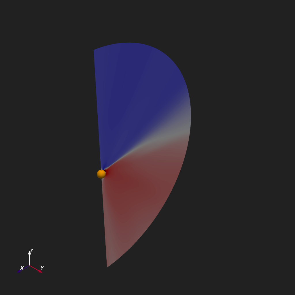
Phi Cut (Meridional Plane)

Fix the longitude at a mid-grid meridian (\(\phi = \phi_{149}\)) and vary both \(r\) and \(\theta\) over their full extents. The resulting surface is a meridional plane that cuts through the full coronal domain, showing the latitudinal and radial structure of \(B_r\) from the solar surface to the outer boundary.

data, r, t, p = read_hdf_by_index(br_file, None, None, 149)

plotter = Plot3d()
plotter.show_axes()
plotter.add_sun()
plotter.add_2d_slice(r, t, p, data * r ** 2, cmap='seismic', clim=(-1, 1),
                     show_scalar_bar=False)
plotter.show()

Static Scene

Interactive Scene