Plotting Magnetic Fieldlines

This example demonstrates add_fieldlines() — the method for rendering traced magnetic fieldlines as spline bundles using mapflpy, the PSI library for integrating along magnetic field data on spherical grids.

run_forward_tracing() and run_fwdbwd_tracing() return a Traces named tuple whose geometry array has shape \((M, 3, N)\):

• \(M\) — the per-fieldline point buffer (NaN-padded to a uniform length).

• \(3\) — spherical coordinate components \((r,\,\theta,\,\phi)\).

• \(N\) — the number of fieldlines.

numpy.moveaxis() transposes this to \((3, M, N)\) so that unpacking with * feeds the three coordinate arrays directly into add_fieldlines.

import numpy as np
from mapflpy.scripts import run_forward_tracing, run_fwdbwd_tracing
from mapflpy.utils import get_fieldline_polarity
from pyvisual import Plot3d
from pyvisual.utils.data import fetch_datasets

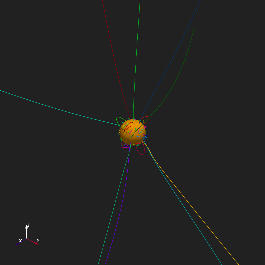
Random Coloring

The simplest coloring strategy assigns a unique random hue to each fieldline via coloring='random'. When no launch_points are supplied, mapflpy places \(n = 128\) seed points quasi-uniformly at \(r = 1.01\,R_\odot\) using the Fibonacci lattice algorithm.

mag_field = fetch_datasets("cor", ["br", "bt", "bp"])
traces = run_forward_tracing(*mag_field, context='fork')
r, t, p = np.moveaxis(traces.geometry, 1, 0)

plotter = Plot3d()
plotter.show_axes()
plotter.add_sun()
plotter.add_fieldlines(r, t, p, coloring='random', line_width=2, show_scalar_bar=False)
plotter.observer_focus = 0, 0, 0
plotter.observer_fov_view = 10
plotter.show()

Static Scene

Interactive Scene

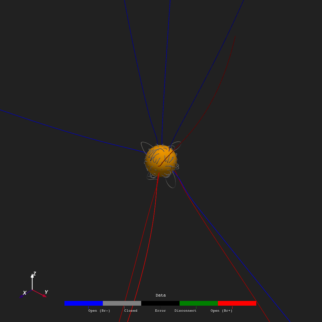
Polarity Coloring

A more informative visualization classifies each fieldline by its open/closed magnetic connectivity via coloring='polarity'. get_fieldline_polarity() evaluates the radial positions of the trace endpoints against the inner (\(r = 1\,R_\odot\)) and outer (\(r = 30\,R_\odot\)) domain boundaries, assigning one of five Polarity states to each line:

• R0_R1_POS — open, \(B_r > 0\) at the inner footpoint.

• R0_R1_NEG — open, \(B_r < 0\) at the inner footpoint.

• R0_R0 — closed, both endpoints anchored at the inner boundary.

• R1_R1 — disconnected, both endpoints at the outer boundary.

• ERROR — unclassified (trace did not reach a boundary).

Combined forward-and-backward traces from run_fwdbwd_tracing() are required so that every fieldline has endpoints on both boundaries, enabling unambiguous polarity assessment.

traces = run_fwdbwd_tracing(*mag_field, context='fork')
polarity = get_fieldline_polarity(1, 30, mag_field.cor_br, traces)
r, t, p = np.moveaxis(traces.geometry, 1, 0)

plotter = Plot3d()
plotter.show_axes()
plotter.add_sun()
plotter.add_fieldlines(r, t, p, polarity, coloring='polarity', line_width=2)
plotter.observer_focus = 0, 0, 0
plotter.observer_fov_view = 10
plotter.show()

Static Scene

Interactive Scene