Polarity-Inversion-Line Seeded Fieldlines

This example traces magnetic fieldlines seeded from the polarity inversion line (PIL) — the curve on the solar surface where the radial magnetic field \(B_r\) changes sign. The PIL marks the boundary between open positive and negative flux and is a natural seed surface for displaying the global topology of the coronal field.

The workflow exploits a key property of SphericalMesh: because it wraps a pyvista.RectilinearGrid whose internal axes store \((r, \theta, \phi)\) directly, PyVista’s pyvista.DataSetFilters.contour() returns a pyvista.PolyData whose points array is already in \((r, \theta, \phi)\) coordinates. This means the contour points can be passed straight to run_fwdbwd_tracing() as launch_points without any intermediate coordinate conversion.

See also Plotting Magnetic Fieldlines for a general introduction to fieldline rendering, and Combining Slices, Contours, and Fieldlines for a broader scene that layers slices, contours, and fieldlines.

import numpy as np
from mapflpy.scripts import run_fwdbwd_tracing
from pyvisual import Plot3d
from pyvisual.core.mesh3d import SphericalMesh
from pyvisual.utils.data import fetch_datasets

Load Data and Extract the Polarity Inversion Line

Build a full SphericalMesh from the coronal \(B_r\) HDF file. Index mesh[5, ...] selects a 2-D spherical shell at radial index 5 — a thin pyvista.RectilinearGrid that spans the full \((\\theta, \\phi)\) domain at a fixed \(r\). The ellipsis (...) expands to fill the remaining two axes.

pyvista.DataSetFilters.contour() with isosurfaces=[0] then finds the iso-curve where \(B_r = 0\) on that shell. The result is the polarity inversion line as a pyvista.PolyData of line segments whose points array holds \((r, \\theta, \\phi)\) coordinates — because the internal axes of SphericalMesh are the spherical coordinates, not Cartesian positions.

mag_field = fetch_datasets("cor", ["br", "bt", "bp"])

mesh = SphericalMesh(mag_field.cor_br)
neutraline = mesh[5, ...].contour(isosurfaces=[0])

Trace Fieldlines from the PIL

run_fwdbwd_tracing() integrates the magnetic field in both the forward and backward directions from each seed point, so that every fieldline has footpoints on both the inner (\(r = 1\,R_{\\odot}\)) and outer (\(r = 30\,R_{\\odot}\)) boundaries. This bidirectional tracing is required for accurate polarity classification and ensures that closed fieldlines connecting two inner-boundary footpoints are also captured.

launch_points=neutraline.points.T passes the PIL vertices directly as the \((3, N)\) seed array in \((r, \\theta, \\phi)\) order. No coordinate conversion is needed because the contour inherits the SphericalMesh coordinate convention.

numpy.moveaxis() transposes the (M, 3, N) geometry array to \((3, M, N)\) so that unpacking with * feeds the three coordinate components directly to add_fieldlines().

traces = run_fwdbwd_tracing(*mag_field, launch_points=neutraline.points.T, context='fork')
r, t, p = np.moveaxis(traces.geometry, 1, 0)

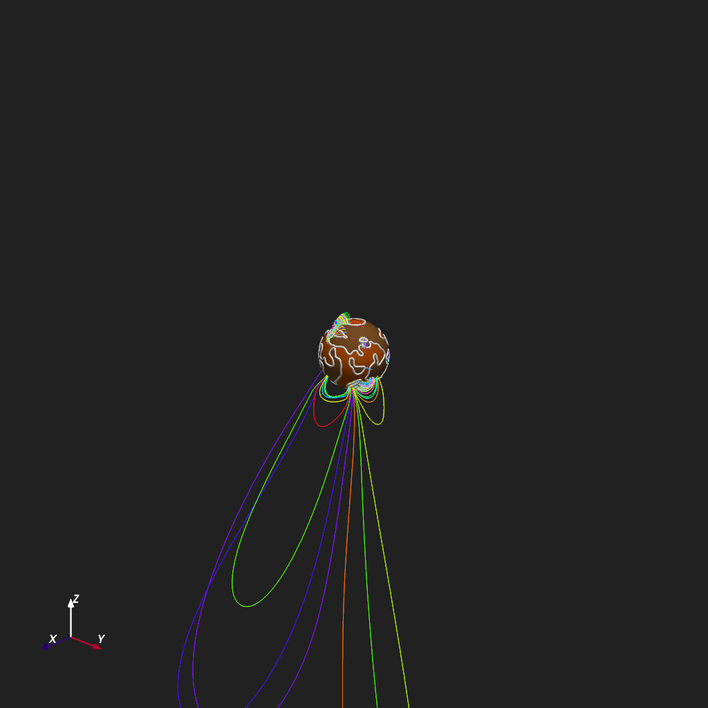
Render the Scene

Three layers are combined in a single Plot3d scene:

• The radial shell mesh[5, ...] coloured by \(B_r\), providing context for the polarity structure at the seed radius.

• The PIL rendered as a white tube, showing the exact seed curve.

• The fieldline bundle, each line assigned a random hue via coloring='random', illustrating the global connectivity of the coronal field anchored at the polarity boundary.

plotter = Plot3d()
plotter.show_axes()
plotter.add_sun()
plotter.add_mesh(mesh[5, ...], cmap='seismic', clim=(-1e-1, 1e-1), opacity=0.5, show_scalar_bar=False)
plotter.add_mesh(neutraline, color='white', line_width=3, render_lines_as_tubes=True)
plotter.add_fieldlines(r, t, p, coloring='random', line_width=1, show_scalar_bar=False)
plotter.observer_focus = 0, 0, 0
plotter.observer_fov_view = 10
plotter.show()

Static Scene

Interactive Scene