1-D Line Slices

This example demonstrates add_1d_slice() — the method for rendering a line slice along a single spherical coordinate axis.

Exactly two of r, t, p must be size-1 arrays, fixing those coordinates. The one array with more than one element defines the slice direction; pyvisual infers the varying axis automatically and renders the result as a polyline colored by the supplied data array.

Real coronal magnetic field data from a PSI MAS model (CR 2282) is loaded via fetch_datasets() and sliced using read_hdf_by_index(). Passing a single integer index for a dimension fixes it to a single grid point; None selects the full extent. The function returns the data and the three coordinate arrays in \((r, \theta, \phi)\) order, ready for direct use with add_1d_slice().

from psi_io import read_hdf_by_index
from pyvisual import Plot3d
from pyvisual.utils.data import fetch_datasets

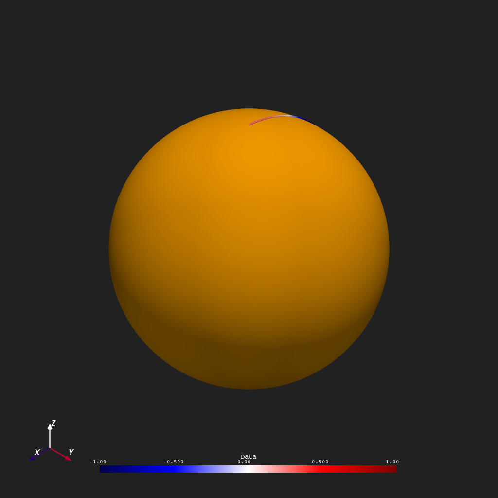
Radial Cut

Fix the colatitude at the equatorial plane (\(\theta = \theta_{71}\)) and a mid-grid longitude (\(\phi = \phi_{149}\)), then sweep radius from the solar surface to the outer coronal boundary. The profile shows how \(B_r\) falls off (and changes sign) with distance from the Sun.

br_file = fetch_datasets("cor", "br").cor_br
data, r, t, p = read_hdf_by_index(br_file, None, 71, 149)

plotter = Plot3d()
plotter.show_axes()
plotter.add_sun()
plotter.add_1d_slice(r, t, p, data, cmap='seismic', clim=(-1, 1), line_width=5)
plotter.show()

Static Scene

Interactive Scene

Theta Cut

Fix the radius near the solar surface (\(r = r_1 \approx 1\,R_\odot\)) and the same mid-grid longitude, then sweep colatitude from the north pole (\(\theta = 0\)) to the south pole (\(\theta = \pi\)). The profile captures the latitudinal structure of \(B_r\) on the inner boundary — sign reversals indicate the boundaries between open-field regions of opposite polarity.

data, r, t, p = read_hdf_by_index(br_file, 1, None, 149)

plotter = Plot3d()
plotter.show_axes()
plotter.add_sun()
plotter.add_1d_slice(r, t, p, data, cmap='seismic', clim=(-1, 1), line_width=5)
plotter.show()

Static Scene

Interactive Scene

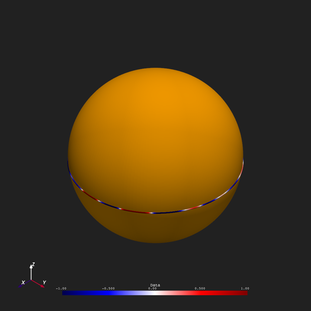
Phi Cut

Fix the same near-surface radius and equatorial colatitude, then sweep longitude \(\phi\) from 0 to \(2\pi\). The resulting ring around the solar equator maps the longitudinal variation of the photospheric \(B_r\) at the equatorial plane — a full-sun longitudinal profile.

data, r, t, p = read_hdf_by_index(br_file, 1, 71, None)

plotter = Plot3d()
plotter.show_axes()
plotter.add_sun()
plotter.add_1d_slice(r, t, p, data, cmap='seismic', clim=(-1, 1), line_width=5)
plotter.show()

Static Scene

Interactive Scene